Non-Terrestrial Networks have two synchronisation problems, not one. The first is timing - signals arrive far later than any terrestrial protocol timer expects, and the delay is different for every UE in the cell. That problem, and the Timing Advance machinery built to solve it, is covered on the NTN Timing Advance page. This page is about the second problem, which is its exact twin in the frequency domain : the satellite is moving fast enough that the carrier frequency the UE receives is not the carrier frequency the network transmitted, and the carrier frequency the network receives is not the one the UE transmitted.

In a terrestrial cell the frequency offset between a UE and a base station is small enough that the receiver's ordinary automatic frequency control loop absorbs it without anyone thinking about it. In NTN it is not. A satellite in low earth orbit moves at roughly 7.6 km/s, which produces a Doppler shift of tens of kilohertz at S band and hundreds of kilohertz at Ka band - values that are larger than a subcarrier spacing, larger than the pull-in range of initial synchronisation, and present in the very first sample the UE ever receives.

The consequence is the same as it was for timing : the large and predictable part of the error has to be removed open loop, computed in advance from the satellite's known trajectory, before the receiver's normal algorithms have any chance of working. This page walks through where the frequency error comes from, how it splits between the UE and the network, how big it actually is in each NTN band, and how accurate the estimate has to be.

• Why Frequency is a Separate Problem from Timing
• Doppler in NTN : the Numbers
• Doppler in Each NTN Operating Band
• Anatomy of the Frequency Error
• Why the UE Cannot Simply Track It
• How the UE Pre-compensates
• What the Network Compensates
• The Timing / Frequency Asymmetry
• Subcarrier Spacing, ICI and How Accurate the Estimate Must Be
• What the Specification Says
• Parameters Involved
• What Breaks When Frequency Compensation is Wrong

Why Frequency is a Separate Problem from Timing

Timing and frequency in NTN come from exactly the same physics - the changing distance between the UE and the satellite - so it is tempting to treat them as one problem with two symptoms. They are closely related, and the relationship is worth knowing precisely, but they are not interchangeable and they are not solved by the same mechanism.

Where they are the same

Doppler shift and delay drift are the same quantity written in different units. A relative velocity expressed as a fraction of the speed of light gives the Doppler shift in parts per million directly, and simultaneously gives the rate at which the one-way propagation delay is changing in microseconds per second :

relative velocity 24 ppm of c  →  Doppler = 24 ppm of the carrier  →  one-way delay changes by 24 us every second

This is why the Doppler figures and the delay-variation figures in TR 38.821 always track each other by a factor of two (the round trip covers the path twice). If you know one, you know the other.

Where they are completely different

NOTE : The last two rows are the ones that matter most in practice. Because the frequency error scales with the carrier, moving an NTN system from S band to Ka band multiplies the problem by roughly a factor of ten while leaving the timing problem untouched. And because there is no network command to correct it, whatever the UE gets wrong stays wrong until the UE itself fixes it.

Doppler in NTN : the Numbers

The Doppler shift for a transmitter and receiver approaching each other at relative velocity v_rel is simply

f_d = ( v_rel / c ) x f_c

so the values quoted in parts per million in the 3GPP reference scenarios convert into hertz the moment a carrier frequency is chosen. What matters is v_rel, the component of velocity along the line of sight - not the satellite's full orbital speed. A satellite passing directly overhead is momentarily neither approaching nor receding, so its Doppler is zero at that instant even though it is moving at 7.6 km/s.

For a 600 km orbit the line-of-sight component peaks at roughly the orbital speed multiplied by R_e/r, i.e. about 6.99 km/s or 23.3 ppm, which is why TR 38.821 quotes 24 ppm as the reference figure.

< Maximum Doppler shift and Doppler rate per orbit, from the TR 38.821 reference scenarios (earth-fixed UE) >

NOTE : These are earth-fixed UE figures - the satellite's contribution alone. A moving UE adds its own term : about 0.46 ppm at 500 km/h, or 1.11 ppm at 1200 km/h (aircraft). Against LEO's 24 ppm that is a few percent and can be treated as part of the residual. Against GEO's 0.93 ppm it is not - an aircraft terminal is then the larger of the two contributions, and it is the one the network cannot predict from ephemeris.

What one pass actually looks like

A table of maxima hides the most important behaviour, which is that the Doppler is not a constant offset but a curve that sweeps from one extreme to the other during a single pass. The plots below are one complete LEO pass, showing slant range, elevation and Doppler together.

< Slant range, elevation angle and Doppler shift over one LEO pass >

NOTE : To vary the altitude, pass geometry and carrier frequency yourself and watch the curves respond, see the 2D Satellite Orbit, Doppler, Distance and Elevation simulator and the Doppler Effect and Propagation Delay tutorial.

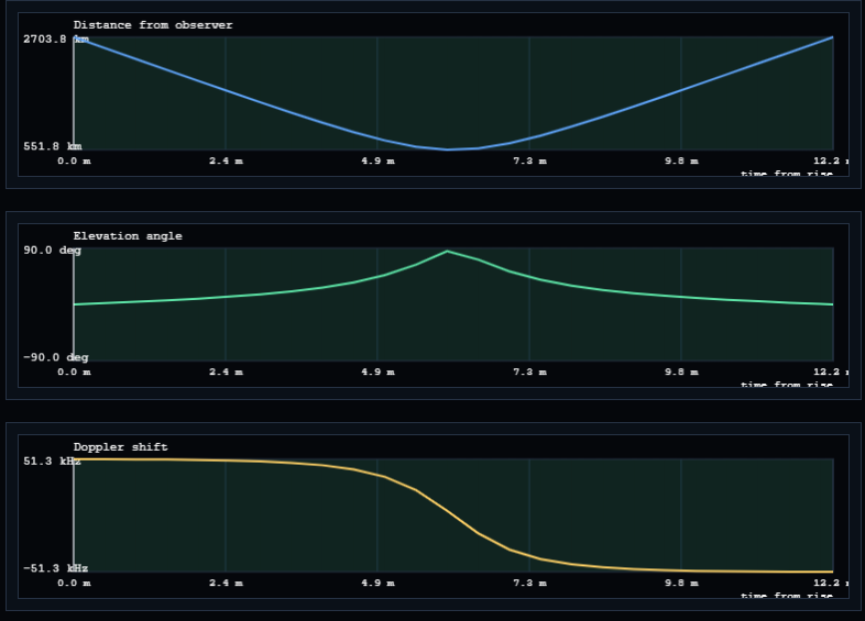
Three features of this picture drive the whole design :

• The Doppler curve is the slope of the distance curve. They are not independent measurements. The zero crossing of the Doppler trace lines up exactly with the minimum of the range trace, because that is the instant the distance stops shrinking and starts growing.
• The full swing is twice the quoted maximum. The Doppler runs from about +51 kHz to about -51 kHz in this example, so the receiver has to cope with a total excursion of over 100 kHz across a pass lasting only twelve minutes.
• The steepest part is in the middle, not at the edges. The Doppler magnitude is largest near the horizon, but its rate of change is largest at closest approach where the shift is passing through zero. A receiver has to survive both, and they occur at opposite ends of the pass.

Doppler in Each NTN Operating Band

Since the Doppler scales with the carrier, the practical size of the problem depends on which NTN band the system uses. The table below applies the LEO 600 km figure of 24 ppm to the band centres defined in TS 38.101-5. The full band definitions are on the NTN Spectrum page.

< Maximum LEO (600 km) Doppler shift per NTN operating band, computed at 24 ppm >

Two conclusions worth carrying away :

• FR2-NTN is an order of magnitude harder in absolute terms. A Ka band uplink can be nearly 700 kHz off frequency for exactly the same orbit that produces 48 kHz at S band. This is one of the reasons the FR2-NTN bands arrived in Rel-18 rather than Rel-17.
• Measured in subcarriers, the gap narrows. FR2 systems use much larger subcarrier spacings, so 450 kHz against a 120 kHz SCS is a similar number of subcarriers as 52 kHz against a 15 kHz SCS. The absolute problem grows with frequency, but the numerology grows with it too - which is exactly why the subcarrier spacing choice matters so much. See Subcarrier Spacing, ICI and How Accurate the Estimate Must Be.

NOTE : n254 is worth a second look. Its downlink sits at 2,483.5 - 2,500 MHz while its uplink sits at 1,610 - 1,626.5 MHz, so the downlink is at a substantially higher frequency than the uplink - the opposite of the usual arrangement. The Doppler is correspondingly larger on the downlink (59.8 kHz) than on the uplink (38.8 kHz), which means the two directions cannot be assumed to need the same correction magnitude.

Anatomy of the Frequency Error

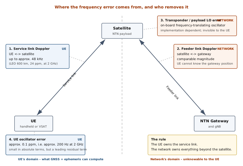
'Doppler' is a convenient single word for what is actually four separate contributions arriving from four different places. Separating them is the key to understanding who is responsible for correcting what, because the answer is different for each one.

< The four frequency error contributions along the UE - satellite - gateway chain >

NOTE : The last row looks negligible next to the first, and in absolute terms it is - 200 Hz against 48 kHz. But it is not negligible against the residual error budget. Once the service link Doppler has been pre-compensated to within a fraction of a percent, the UE's own oscillator becomes one of the dominant remaining error terms. The interesting engineering question in NTN frequency compensation is rarely 'can we remove the Doppler' - it is 'what is left after we have'.

The split mirrors the timing split exactly

Notice that the ownership column reproduces the arrangement described on the NTN Timing Advance page : the UE owns the service link, the network owns everything beyond the satellite. This is not a coincidence but a direct consequence of what each party can possibly know. The UE has GNSS and the broadcast ephemeris, which is exactly the information needed to compute the service link geometry and nothing else. Everything on the far side of the satellite is invisible to it, in both the time and frequency domains.

Why the UE Cannot Simply Track It

A reasonable first reaction is that receivers have always had automatic frequency control, so why is a special mechanism needed at all ? The answer has two parts, and the first one is decisive.

1. The offset is present before synchronisation begins

An AFC loop can only correct an offset once it has acquired the signal. Initial acquisition in NR happens on the PSS and SSS, and the frequency error that this process can absorb without additional hypothesis testing is on the order of half a subcarrier spacing - a few kilohertz at 15 kHz SCS. Compare that with the numbers from the previous section :

In every case the raw Doppler is several times larger than the acquisition range. A UE that simply powered on and searched would not merely acquire the cell inaccurately - it would not find the cell at all. The large part of the offset therefore has to be removed before the search starts, which means it has to be computed rather than measured.

2. Locking to the downlink gives the wrong uplink correction

This one is subtle and is worth working through carefully, because it explains why an explicit uplink pre-compensation is required even for a UE that is already perfectly tracking the downlink.

In NR the UE derives its uplink carrier frequency from the downlink it receives. Suppose the satellite is approaching, so the downlink arrives shifted up by f_d. A UE that locks its oscillator to that downlink will also transmit shifted up by the corresponding amount. The uplink signal then travels the same closing path and picks up another upward shift on the way to the satellite. The result at the satellite receiver is not zero error - it is roughly twice the Doppler :

naive downlink locking  →  error at the satellite ≈ 2 f_d   (not 0)

In a terrestrial cell this doubling is harmless because f_d is a few hundred hertz at worst. In LEO it turns a 48 kHz problem into a 96 kHz one. The UE must therefore apply a deliberate correction in the opposite direction on its transmitter, sized so that the signal arrives at the satellite on the nominal frequency. That correction cannot be derived from the downlink - it has to come from the geometry.

How the UE Pre-compensates

The good news is that the UE already has everything it needs, because it is the same input set the Timing Advance calculation uses. No additional signalling and no additional hardware is required beyond what NTN timing already demands.

• Its own position and velocity, from GNSS. NTN access requires a valid GNSS fix in any case.
• The satellite's position and velocity, from ephemerisInfo in SIB19 - supplied either as Cartesian state vectors (positionVelocity) or as classical orbital elements (orbital).
• A common time reference, from epochTime, so that both sets of coordinates refer to the same instant.

From these the UE forms the relative velocity vector, projects it onto the line of sight to obtain v_rel, and applies f_d = (v_rel/c) f_c - separately for the downlink and uplink carriers, since in an FDD band those are different frequencies and therefore different shifts.

< Projection of the satellite velocity onto the line of sight >

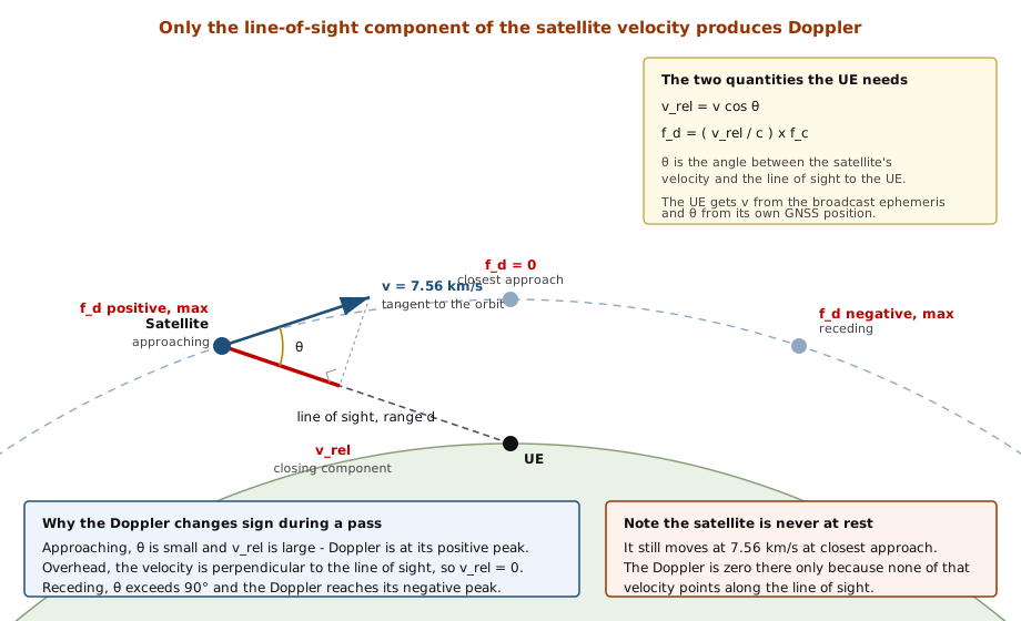
This is the geometry behind every number on this page, and it explains the one feature of the Doppler curve that surprises people : the satellite is moving at 7.56 km/s at closest approach just as it is everywhere else, yet the Doppler there is exactly zero. Nothing has slowed down - it is simply that at that instant none of the velocity points along the line of sight, so the range is momentarily stationary even though the satellite is not.

One geometry calculation, two corrections

It is worth being explicit that the timing and frequency pre-compensations are not two separate computations. The UE computes the UE-to-satellite geometry once, and reads two different quantities off it :

This is why the two problems are always discussed together and why one set of assistance data serves both. It is also why the validity rules are shared : when ntn-ULSyncValidityDuration expires, the UE loses its right to transmit not because its timing has gone stale but because its whole geometric picture has - and the frequency estimate is just as stale as the timing one.

What the Network Compensates

Everything beyond the satellite is the network's responsibility, and the important architectural point is that the network does this work silently. There is no broadcast field telling the UE about the feeder link Doppler, in the way that ta-Common tells it about the feeder link delay. The correction is applied before the signal ever reaches the UE, so from the UE's point of view it simply does not exist.

• Feeder link Doppler is pre-compensated at the gateway on transmit and post-compensated on receive. The gateway knows the satellite's ephemeris and its own fixed position exactly, so this is a straightforward calculation for it - considerably easier than the UE's, since neither endpoint is uncertain.
• Transponder frequency error - the accuracy of the payload's frequency-translating oscillator - is likewise handled on the ground, typically by monitoring a reference signal through the payload and correcting for the observed offset.

Why a transparent payload makes this harder

In a regenerative system the satellite demodulates and regenerates the signal, so the feeder link and the service link are separate frequency problems that never interact. The service link is generated fresh on board at the correct frequency.

In a transparent system the satellite is an analogue repeater, so whatever frequency error exists on the feeder link is relayed straight through onto the service link and lands on the UE. The gateway therefore has to pre-distort its transmission so that after the feeder link Doppler, the frequency translation on board, and the payload's own oscillator error, the signal arrives at the UE on the nominal carrier. This is the frequency-domain equivalent of the Common TA, but it is solved entirely on the network side instead of being shared with the UE.

NOTE : This asymmetry with the timing case is deliberate and worth understanding. Timing could not be handled this way - the network cannot pre-compensate the propagation delay towards every UE individually, because a single downlink transmission serves the whole beam and the UEs are at different distances. Frequency can be handled this way for the feeder link, because the feeder link is a single point-to-point path shared by everyone in the beam. What is common to all UEs can be removed by the network; what differs per UE must be left to the UE.

The Timing / Frequency Asymmetry

Having gone through both mechanisms, the differences between how 3GPP handles timing and how it handles frequency are striking - and they are worth tabulating, because a lot of confusion comes from assuming the two are handled symmetrically.

The fourth row is the one that surprises people most. There is no frequency equivalent of the Timing Advance Command. NR simply does not have a mechanism by which a gNB tells a UE to shift its transmit frequency by a specified amount - it never needed one, because a terrestrial UE that locks to the downlink is automatically close enough. NTN inherited that absence, and closed the gap by making the UE compute its own correction rather than by inventing a new command.

This has a practical consequence for anyone debugging an NTN link : a timing problem tends to be self-correcting once random access succeeds, because the network keeps issuing corrections. A frequency problem does not self-correct. If the UE's Doppler estimate is wrong, nothing in the protocol will tell it so.

Subcarrier Spacing, ICI and How Accurate the Estimate Must Be

Pre-compensation never removes the error completely. What matters is whether what remains is small enough, and 'small enough' in an OFDM system means small compared with the subcarrier spacing. A residual frequency offset destroys the orthogonality between subcarriers and shows up as inter-carrier interference (ICI), which behaves like a noise floor that no amount of transmit power can overcome.

A common engineering rule of thumb is to keep the residual below roughly 1 to 2 % of the subcarrier spacing for the ICI to stay negligible. That converts into a concrete budget :

What that means for the ephemeris accuracy

A 99.7 % accuracy requirement sounds alarming until it is converted back into the physical quantity the UE actually estimates. At 2,185 MHz, a residual of 150 Hz corresponds to

150 Hz / 2,185 MHz = 0.069 ppm  →  v_rel error of about 20 m/s

In other words the UE's estimate of the line-of-sight closing velocity has to be good to about 20 metres per second, out of roughly 7,000 m/s. That is a very mild requirement - GNSS velocity and broadcast ephemeris comfortably do far better. The same calculation for the timing side gives a required range accuracy of a few hundred metres, which is equally undemanding.

This is the reassuring conclusion of the whole page, and it is worth stating plainly : NTN frequency compensation is not hard because the arithmetic is delicate. It is hard because it has to happen before the receiver is working at all, and because nothing in the protocol will tell the UE if it gets it wrong. Once the UE has a valid GNSS fix and valid ephemeris, the accuracy takes care of itself. The engineering effort goes into making sure it always has them.

NOTE : Notice that the residual budget at 15 kHz SCS is around 150 Hz, while a typical UE oscillator accuracy of 0.1 ppm at 2 GHz is around 200 Hz. These are the same order of magnitude, which reinforces the point made earlier - after a good pre-compensation the UE's own oscillator is not a negligible term but one of the leading ones.

What the Specification Says

It is worth separating what is described in the study documents from what is actually required of a UE, because frequency compensation is an area where 3GPP specifies the outcome rather than the method.

• TR 38.811 characterises the Doppler behaviour of the various orbits and establishes the magnitudes the system has to live with.
• TR 38.821 studies the compensation options and settles the split of responsibility between the UE and the network.
• TS 38.300 states the normative behaviour : a UE with a valid GNSS position and valid ephemeris pre-compensates the frequency Doppler on the service link, while Doppler on the feeder link and any transponder frequency error are handled by the network.
• TS 38.101-5 carries the RF requirements - the frequency error the UE must actually achieve, which is the requirement a test house will measure. 3GPP does not specify how the UE computes the correction, only how accurate the result has to be.

What the frequency error requirement is measured against

The detail that matters more than the numeric value is the reference. In terrestrial NR the UE's modulated carrier frequency accuracy is specified as approximately +/- 0.1 ppm relative to the carrier frequency received from the base station, observed over one slot - not against an absolute frequency standard. The UE is therefore allowed to be off in absolute terms, provided it faithfully follows whatever it receives.

In NTN that reference is a moving target, because the carrier the UE receives is itself Doppler-shifted. Following the downlink faithfully is no longer the same thing as transmitting on the frequency the satellite expects - in fact, as shown in Why the UE Cannot Simply Track It, following it faithfully produces roughly twice the error at the satellite. This is the structural reason the pre-compensation has to be a deliberate, explicitly computed action rather than a by-product of the tracking loop.

The current numeric requirements for satellite access are in TS 38.101-5, and they are worth reading from the live version of the specification rather than from any secondary source, since they have been extended as the FR2-NTN bands were added.

Why the oscillator specification matters more in NTN than in a terrestrial network

A 0.1 ppm oscillator sounds like a solved problem, and in a terrestrial network it is. In NTN it is worth converting into hertz per band and comparing it with the ICI budget from the previous section, because the answer is not what intuition suggests.

< UE oscillator accuracy of 0.1 ppm expressed in hertz, against a 1 % of subcarrier spacing ICI budget >

The pattern is striking. Across every NTN band, a UE oscillator sitting exactly at its 0.1 ppm limit already consumes the whole 1 % ICI budget on its own - and at Ka band it consumes more than twice it, even against a 120 kHz subcarrier spacing. The Doppler pre-compensation has not even been considered yet at this point.

Two things follow from that, and they are the practical conclusion of this whole page :

• The 1 % figure is a rule of thumb, not a limit. Real systems clearly operate with residuals larger than 1 % of the subcarrier spacing, because the oscillator specification alone guarantees it. ICI degrades gracefully rather than falling off a cliff, and a few percent is tolerable.
• One-shot pre-compensation is never enough. Because the floor is set by hardware the UE cannot compute away, the receiver has to keep tracking the residual continuously with its normal frequency loops. Pre-compensation exists to bring the error down from tens of kilohertz to something those loops can handle - not to eliminate it. That is the correct mental model : open loop gets you into range, closed loop keeps you there.

Release timeline

• Rel-17 : first normative NR-NTN. Transparent payload only, FR1-NTN bands only, and GNSS capability required of the UE - which is what makes the whole pre-compensation approach possible.
• Rel-18 : NTN extended above 10 GHz into the FR2-NTN bands. As the table in Doppler in Each NTN Operating Band shows, this multiplies the absolute frequency error by roughly ten, which is a large part of why it was a separate release.
• Rel-19 and beyond : continued NR-NTN and IoT-NTN enhancements. The frequency compensation architecture - UE owns the service link, network owns the rest - has remained stable throughout.

Parameters Involved

The striking thing about this table is how short it is compared with the timing equivalent on the NTN Timing Advance page. There is no frequency counterpart to ta-Common, no drift terms, no offsets and no reports - because the network handles its own share silently rather than delegating it.

The ASN.1 detail for all of these is on the NTN RRC (NR) page.

What Breaks When Frequency Compensation is Wrong

Frequency faults have a distinctive signature : they tend to produce a link that either does not exist at all or that degrades in a way that looks like poor coverage but does not improve with more power.

NOTE : The two elevation-dependent rows are the most useful diagnostic pair on this page. If a link is worst in the middle of a pass, the problem is the Doppler rate and the tracking loop. If it is worst at the edges, the problem is the Doppler magnitude and the pre-compensation range. The same fault would be indistinguishable from a coverage problem without knowing where in the pass it occurred.

Related Pages on this Site

• NTN Timing Advance - the time-domain twin of this page, and the source of the geometry the frequency calculation reuses
• NTN Spectrum - the FR1-NTN and FR2-NTN band definitions used in the per-band Doppler table
• NTN RRC (NR) - the SIB19 and ntn-Config ASN.1 behind ephemerisInfo and epochTime
• NTN RACH - where an uncorrected frequency error shows up first, since the preamble is the UE's first transmission
• NTN Architecture - why a transparent payload relays the feeder link frequency error straight through to the UE
• NTN Challenges - Doppler seen alongside the other NTN problems
• Web Simulator : 2D Satellite Orbit, Doppler, Distance and Elevation - vary the orbit and carrier and watch the Doppler curve respond
• Web Simulator : Doppler Effect and Propagation Delay - the underlying relationship without the orbital geometry

3GPP Reference

• Non-Terrestrial Networks (NTN) - 3GPP Technology Article (2024)
• 3GPP TR 38.811 : Study on New Radio (NR) to support non-terrestrial networks - Doppler characterisation per orbit
• 3GPP TR 38.821 : Solutions for NR to support non-terrestrial networks (NTN) - reference scenario Doppler and Doppler variation figures
• 3GPP TS 38.300 : NR and NG-RAN Overall Description - clause 16.14, UE frequency pre-compensation and the UE / network split
• 3GPP TS 38.101-5 : NR; UE radio transmission and reception; Part 5: Satellite access - UE frequency error requirements and the NTN operating bands
• 3GPP TS 38.101-1 : NR; UE radio transmission and reception; Part 1: Range 1 Standalone - the terrestrial frequency error requirement for comparison
• 3GPP TS 38.211 : NR; Physical channels and modulation - subcarrier spacings and numerologies
• 3GPP TS 38.331 : NR; Radio Resource Control (RRC) protocol specification - SIB19, ntn-Config, EphemerisInfo and epochTime
• 3GPP TR 36.763 : Study on NB-IoT / eMTC support for Non-Terrestrial Networks - the IoT-NTN counterpart, where the Doppler-to-subcarrier ratio is far more severe

Other References

• Non-terrestrial networks (NTN) - R&S
• Non-Terrestrial Network Advantages, Challenges, and Applications - Keysight
• 5G & Non-Terrestrial Networks - 5G Americas White Paper (2022)
• Orbit of a satellite Calculator
• LEO Small-Satellite Constellations for 5G and Beyond-5G Communications
• Satellite Communications in the New Space Era: A Survey and Future Challenges
• 5G from Space: An Overview of 3GPP Non-Terrestrial Networks