Timing Synchronization

Communiation through Satellites in NTN introduces significant challenges in timing and synchronization due to the large distances involved, which result in much longer propagation delays compared to terrestrial networks. For example, a satellite in geostationary orbit (GEO) at ~36,000 km altitude introduces a round-trip time (RTT) of about 240 ms, whereas terrestrial networks typically have RTTs of a few milliseconds.

In NTNs, the large distances and relative motion between the UE and the satellite introduce significant challenges in timing, synchronization, and frequency alignment. This section of the 3GPP specification ensures that the UE and network can communicate reliably by:

• Adjusting for propagation delays using offsets and Timing Advances.
• Managing HARQ processes to handle long RTTs.
• Pre-compensating for Doppler shifts to maintain frequency alignment.

This is critical for applications like satellite-based internet (e.g., Starlink), remote sensing, and global IoT connectivity, where NTNs are increasingly important.

The note addresses how to manage these delays to ensure proper communication between the UE (e.g., a smartphone or IoT device), the gNB (on the satellite), and the NTN gateway (on Earth), especially when the gNB and NTN gateway are co-located.

• Why Timing in NTN is a Different Problem
• Scheduling and Timing
• Reading the Timing Relationship Diagram
• The Timing Advance Equation
• Common TA, Drift and Validity
• K_offset and K_mac in Practice
• HARQ Operation
• Why HARQ Stalls in NTN - in Numbers
• Timing Advance and Frequency Pre-compensation
• Doppler in Numbers
• TA Lifecycle : Acquire, Apply, Maintain
• Worked Example : Where the 3GPP Numbers Come From
• Where the Numbers Live : SIB19 Parameters
• What Breaks When the Timing is Wrong

Why Timing in NTN is a Different Problem

It is tempting to think of NTN timing as 'terrestrial timing, but with bigger numbers'. It is not, and the reason is worth being precise about. Timing advance exists in LTE and NR too, so the mechanism is familiar - but in a terrestrial cell the delay is small, almost constant, and measurable by the network from the very first preamble. In NTN none of those three things is true, and each one that breaks forces a different piece of machinery into the specification.

NOTE : The terrestrial column is not a claim that terrestrial channels are static. NR is specified for UE speeds up to 500 km/h, and high-speed train scenarios are a well developed part of the terrestrial requirements. The comparison is about magnitude and about ownership :

• Magnitude. A UE at 500 km/h has a relative velocity of 0.46 ppm of c. A LEO satellite at 600 km reaches 24 ppm. Even the fastest train is therefore around fifty times below the LEO figure, and that is before remembering that in NTN the satellite's own motion is present in addition to whatever the UE is doing. At GEO the picture inverts : a UE at 1200 km/h (1.11 ppm) actually contributes more Doppler than the satellite's 0.93 ppm, so for GEO the terrestrial intuition about UE mobility is the right one.
• Ownership, and therefore predictability. In a terrestrial cell the motion belongs to the UE, so the network cannot predict it and the receiver has to track it closed-loop. In NTN the dominant motion belongs to the platform, whose trajectory is known in advance and broadcast as ephemeris. That is precisely why open-loop pre-compensation is possible at all in NTN and is not a technique terrestrial NR ever needed.

There is one quantity where the terrestrial case is genuinely not the milder one, and it is worth stating so the comparison is honest. The Doppler rate of change peaks at closest approach, where it is approximately v² f_c / (d₀ c) for a UE passing a site at distance d₀. A train at 500 km/h passing within 50 m of a trackside site sees roughly 2.6 kHz/s at 2 GHz - several times the 540 Hz/s of a LEO pass, because the geometry changes far more abruptly at 50 m than at 600 km. Terrestrial receivers have therefore always coped with fast Doppler dynamics. What they have never had to cope with is a Doppler offset of tens of kilohertz that is already present in the very first sample, before synchronisation has started - and that, rather than the rate of change, is the specifically NTN problem.

Three separate problems hiding behind one word

Almost every NTN timing feature in the specification can be traced back to one of these three, and it is much easier to keep them straight than to treat 'delay' as a single issue :

• 1. The absolute delay is huge. This is a large, essentially common offset shared by everyone in the cell. It does not stop the radio link from working, but it breaks every protocol relationship that assumes a response arrives 'a few slots later' - scheduling offsets, response windows, MAC CE application timing and HARQ round trips. The answer is the Common TA plus the scheduling offsets K_offset and K_mac, and the option to stop relying on HARQ feedback altogether.
• 2. The delay is different for every UE in the cell. A UE at the centre of a 1,000 km footprint and one at its edge are milliseconds apart - far more than a cyclic prefix. A single common correction therefore cannot align everybody, which is why NTN keeps a UE-specific TA term on top of the common one, and why the UE has to compute its own before its first transmission. This is also the part that makes the RACH design hard - see NTN RACH.
• 3. In LEO, the delay will not sit still. At 7.56 km/s(linear speed of the satellite in 600km orbit as an example), the round trip time changes by tens of microseconds every second, so a TA value is not a setting - it is a trajectory. This is why the network broadcasts not just a common TA but its first and second derivatives (drift and drift variant), and why the assistance data comes with a validity duration after which it must be refreshed.

Where the 7.56 km/s comes from

That figure is quoted in TR 38.821 Table 7.1-1 as the relative speed of the satellite with respect to the earth for the 600 km scenarios, but it is worth knowing that it is nothing more than the circular orbit velocity :

v = sqrt( μ / r ) = sqrt( 398,600 / 6,971 ) = 7.56 km/s

with μ = 398,600 km³/s² the Earth's standard gravitational parameter, and r the orbital radius measured from the centre of the Earth - so r = 6,371 + 600 = 6,971 km for a 600 km altitude, not 600 km. The same formula gives 7.26 km/s at 1,200 km and 3.07 km/s at GEO.

From orbital speed to delay drift

For timing purposes what matters is not the full 7.56 km/s but its component along the line of sight, because only that changes the path length. That component is largest when the satellite is low on the horizon and falls to zero as it passes directly overhead - which is why the delay drift changes sign during a pass. Two useful bounds follow :

• The range rate can never exceed the orbital speed itself, so the Doppler is hard-limited to 7.56 / 299,792 = 25.2 ppm. Nothing in a 600 km LEO system can be faster than that.
• Geometrically the line-of-sight component maxes out at roughly v x R_e / r near the horizon, i.e. around 23 ppm. TR 38.821 quotes 24 ppm for the reference scenario, comfortably inside the bracket.

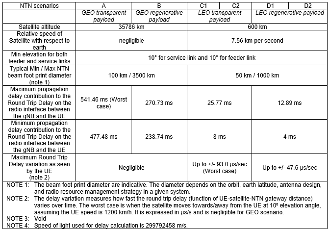
And that is where the 'tens of microseconds every second' in the bullet above comes from. A range rate of about 24 ppm means the one-way path length changes by about 24 us of propagation time per second, so the round trip delay drifts at roughly 48 us/s - which is exactly the +/- 47.6 us/s that Table 7.1-1 lists for the LEO regenerative scenarios. The Doppler row and the delay-variation row of that table are the same physical quantity written in two different units, as noted in Doppler in Numbers below.

What this actually looks like over a single pass

All of the above is much easier to see than to describe. The three plots below are one complete LEO pass - the satellite rising at the horizon, going almost directly overhead, and setting again - with slant range, elevation angle and Doppler shift plotted against time from rise.

< Slant range, elevation angle and Doppler shift over one LEO pass >

NOTE : For playing with this yourself - changing the altitude, the elevation of the pass or the carrier frequency and watching all three curves respond - see the 2D Satellite Orbit, Doppler, Distance and Elevation simulator. The Doppler Effect and Propagation Delay tutorial covers the underlying relationship on its own.

Reading the three plots together

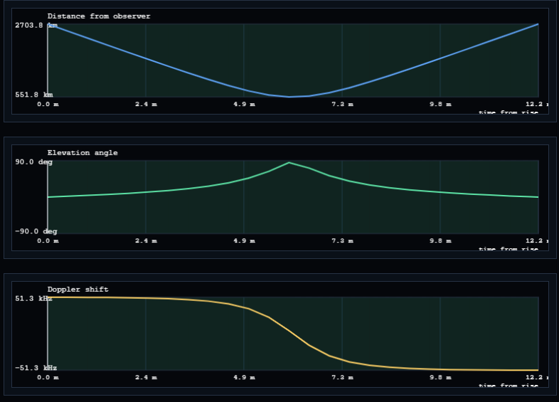
The single most important thing in this picture is that the Doppler curve is the slope of the distance curve. They are not two independent measurements - the middle plot tells you where you are in the pass, the top plot is the delay, and the bottom plot is its rate of change. Once that clicks, everything else on this page follows :

• Distance (top) starts at 2,703.8 km at the horizon, falls to 551.8 km at closest approach, and climbs back. In timing terms the round trip delay swings from about 18.0 ms down to 3.7 ms and back up - a 14.4 ms change, on the same link, with the same satellite, in about six minutes. No single TA value could possibly serve that pass, which is exactly why the assistance data is a polynomial with a validity duration rather than a number.
• Elevation (middle) rises from 0° to nearly 90° and back over 12.2 minutes. That is the whole visibility window for one satellite - and it is the practical reason a LEO cell has to be handed over every few minutes whether or not the UE ever moves.
• Doppler (bottom) starts at its positive maximum of +51.3 kHz while the satellite is approaching, passes through exactly zero at the moment of highest elevation, and ends at -51.3 kHz as the satellite recedes. The zero crossing lines up precisely with the minimum of the distance curve, because that is the instant the range stops shrinking and starts growing.

Cross-checking the plot against the specification numbers

This particular pass is a useful worked example because every value in it can be reproduced from the formulas above. The 2,703.8 km maximum is the slant range at 0° elevation for a 550 km orbit - sqrt(2 x 6,371 x 550 + 550²) = 2,703.8 km - and 551.8 km is very nearly the altitude itself, as it must be for a near-overhead pass. At 550 km the orbital speed is sqrt(398,600 / 6,921) = 7.59 km/s, giving a horizon-to-horizon transit of about 12.2 minutes, which is what the time axis shows.

• The peak line-of-sight velocity is v x R_e / r = 7.59 x 6,371 / 6,921 = 6.99 km/s, i.e. 23.3 ppm - right in the middle of the 23 to 25.2 ppm bracket derived above, and consistent with the 24 ppm that TR 38.821 quotes for its 600 km reference case.
• Working backwards from the plot, a peak of 51.3 kHz at 23.3 ppm implies a carrier of about 2.2 GHz - S band, at the top of NTN band n256. Change the carrier and the top two plots stay exactly where they are while the bottom one scales linearly, which is a good way to convince yourself that Doppler is a frequency-domain restatement of the same geometry.
• The corresponding round trip delay drift is 2 x 23.3 = 46.6 us/s at the horizon, against the +/- 47.6 us/s that Table 7.1-1 lists for LEO regenerative scenarios. The plot and the specification table are describing the same thing.

NOTE : Look at where the Doppler curve is steepest - it is not at the edges where the shift is largest, but in the middle, at closest approach, where the shift is passing through zero. That is the Doppler rate maximum discussed earlier, and it is the same effect that makes a high-speed train passing close to a trackside site a demanding case terrestrially. The magnitude of the offset and the rate of change of the offset peak at opposite ends of the pass, and a receiver has to survive both.

NOTE : 7.56 km/s is the speed of the satellite in orbit, which is not the speed at which its beam footprint sweeps across the ground. The sub-satellite point moves at v x R_e / r, about 6.9 km/s. Use 7.56 km/s for Doppler and delay drift as on this page, and 6.9 km/s when working out how long a moving beam dwells over a given place - see NTN Architecture.

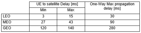
< TR38.811 - typical one-way propagation delay per orbit >

< TR38.821 v16.2.0-Table 7.1-1: Propagation delay and delay variation per NTN scenario >

NOTE : Notice in this table that the delay figures for the transparent scenarios (A, C1, C2) are exactly twice those of the corresponding regenerative ones (B, D1, D2), and so is the delay variation. That is not a coincidence - in a transparent system the feeder link is inside the UE's radio round trip, in a regenerative system it is not. The payload type therefore changes the timing problem before any protocol design starts. See NTN Architecture for why.

Scheduling and Timing

In NTNs, scheduling and timing are critical due to the significant propagation delays introduced by long distances between UE and satellite-based gNBs. To maintain synchronization between downlink (DL) and uplink (UL) transmissions, frame alignment is achieved at the uplink time synchronization reference point (RP), with adjustments made using a configured offset. To address timing discrepancies and ensure accurate scheduling, the system incorporates a Common Timing Advance (Common TA) along with two additional timing offsets: K_offset and K_mac. These parameters collectively compensate for round-trip delays and allow sufficient processing time for the UE between DL reception and UL transmission. Furthermore, they facilitate proper coordination in procedures such as random access and MAC CE command handling, ensuring that frame alignment and resource scheduling remain robust despite the inherent latency of NTN environments.

Timing Advance and additional terminologies related to NTN Timing Adjustment are well summarized in the following diagram.

< 38.300 - Figure 16.14.2.1-1: Illustration of timing relationship (for collocated gNB and NTN Gateway) >

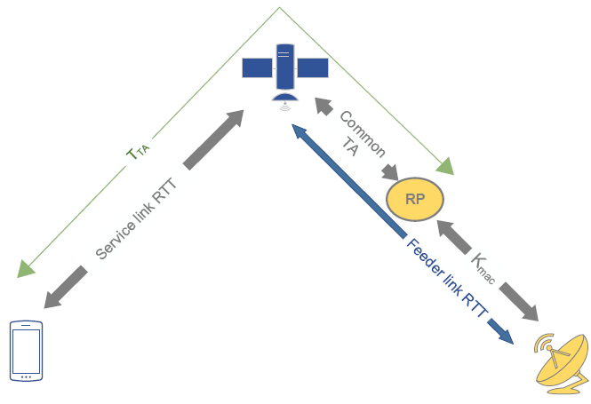
• Service Link RTT: The delay between the UE (on Earth) and the satellite.
• Feeder Link RTT: The delay between the satellite and the NTN gateway (on Earth).
• Common TA: The RTT between the RP and the NTN payload.
• T_TA: The total timing advance, which includes the service link RTT and feeder link RTT.
• K_mac: The offset applied to account for the RTT between the RP and gNB.

Following is breakdown of each component on the diagram and its definition.

• Uplink (UL) Frame Alignment and Timing Reference Point (RP):
• The UE aligns its uplink (UL) frame timing with the reference point (RP) on the satellite (gNB), adjusted by an offset called N_TA,offset. This offset accounts for the propagation delay between the UE and the satellite.
• Propagation Delay in NTNs:
• Due to the large distances in NTNs, the propagation delay is significant. To manage this, the system uses a Common Timing Advance (Common TA) and two offsets: K_offset and K_mac.
• Timing Relationships:
• Common TA: This is the round-trip time (RTT) between the RP (on the satellite) and the NTN payload (also on the satellite). Since the gNB and NTN gateway are co-located, this RTT represents the delay between the satellite and the ground gateway.
• K_offset: A scheduling offset that must be at least equal to the sum of the service link RTT (between UE and satellite) and the Common TA. It ensures the UE has enough time to process downlink receptions and uplink transmissions. (Must be >= RTT of Service Link + Common TA.)
• K_mac: Another offset, approximately equal to the RTT between the RP and the gNB (on the satellite). It allows the UE sufficient processing time for downlink and uplink tasks.
• Practical Configuration:
• The offset K_offset is used to give the UE enough time to process downlink data and prepare uplink transmissions.
• K_mac is used to determine the start of the Random Access Response (RAR) window or MsgB window after a Msg1/MsgA transmission (part of the random access procedure).

Is the RP a physical entity ?

This is the first question almost everyone asks about the diagram, and the answer is worth stating plainly : no. There is no equipment at the RP. Nothing is installed there, nothing transmits from there, and no vendor sells one.

The RP is a timing definition - the point at which uplink frame timing is defined to be aligned with downlink frame timing (offset by N_TA,offset). TS 38.300 calls it the uplink time synchronization reference point and never ties it to any physical entity.

The detail that settles it is this : the UE is never told where the RP is. No field in SIB19 carries its position. The only thing that reaches the UE is ta-Common, the round trip between the RP and the satellite. So the RP's location is defined by that broadcast number rather than the other way round.

Notice how 3GPP drew it in the figure : the RP is a blob floating on the feeder link, deliberately not on the satellite and not on the dish. That is the specification's way of saying it is neither of them.

A useful analogy : the calibration plane

If you have ever calibrated a vector network analyser, you already know this concept. You calibrate to a reference plane that may sit in the middle of a cable where there is no connector, no component and nothing to point at - yet every measurement afterwards is expressed relative to it, and moving the plane changes all your numbers without changing a single piece of hardware. The RP is exactly that idea applied to timing instead of to S-parameters.

Why define such an abstraction at all ?

Because it decouples the specification from the deployment. Since the split between 'what the network broadcasts' and 'what the UE computes' is expressed relative to a movable reference rather than a named box, the same set of timing equations describes both a transparent payload with a ground-based gNB and a regenerative payload with the gNB in orbit. No separate specification text is needed per architecture. It is the same instinct that leads TS 38.101-5 to talk about a 'Satellite Access Node' rather than naming the satellite or the gateway.

NOTE : Logical does not mean arbitrary. Whatever value the operator broadcasts must be consistent with the real feeder link geometry. If it is not, every UE in the cell pre-compensates towards a point that does not match reality, and their transmissions arrive misaligned by exactly the amount of the error. You may put the RP anywhere you like; you may not then be wrong about the distance to it.

NOTE : One point of care when reading the bullet list above - the RP is drawn on the feeder link, not on the satellite. If the RP were literally at the satellite then Common TA would be zero by definition, since Common TA is the round trip between the RP and the NTN payload. A non-zero Common TA means precisely that the RP sits beyond the payload on the feeder side. In the collocated gNB-and-gateway case drawn in the figure, the RP is effectively at the gateway, which is why Common TA equals the feeder link RTT and K_mac collapses to zero.

The same diagram, with numbers

The terms above stay abstract until they are given values, so here is the whole figure filled in for three concrete deployments, using the worst-case (10° elevation) reference figures from TR 38.821 that appear elsewhere on this page. Every row is just the diagram read with a different RP placement and a different orbit.

Three things become obvious once the diagram carries numbers rather than labels :

• T_TA is not the same as the service link RTT. In the transparent columns it is twice as large, because the UE is compensating for a feeder link it cannot see and knows nothing about. This is the single most common misreading of the figure.
• Moving the RP moves work between the two parties, not out of the system. Compare the two LEO columns : the regenerative case has a Common TA of zero, but the feeder link has not vanished - it has simply been placed outside the UE's timing loop, where the network deals with it alone.
• K_mac is zero in all three columns, because all three assume the gNB sits at the RP. It only becomes non-zero in the case the figure's caption explicitly excludes - a gNB that is not collocated with the gateway, for instance one gNB serving several gateways over terrestrial transport.

Reading the Timing Relationship Diagram

The 38.300 figure above repays a slow reading, because almost every NTN timing term is defined by which two points on that picture an arrow spans. There are three physical nodes in it - the UE at bottom left, the satellite at the top, the NTN gateway at bottom right - and one node that is not physical at all.

The Reference Point (RP) is not a place

The yellow ellipse marked RP sits on the feeder link, between the satellite and the gateway, and it is the single most misunderstood object in the diagram. It is not a piece of equipment. It is a definition : the point in the chain at which uplink frame timing is defined to be aligned with downlink frame timing (offset by N_TA,offset). Every other quantity in the picture is expressed relative to it :

• Service link RTT spans UE <-> satellite. The UE has to work this one out for itself, because only the UE knows where it is.
• Common TA spans RP <-> NTN payload. This is the part every UE in the cell shares, so the network can simply broadcast it.
• Feeder link RTT spans satellite <-> gateway. Part of it is inside the Common TA and part of it is beyond the RP, depending on where the RP is placed.
• K_mac spans RP <-> gNB. In the figure the gNB and the gateway are collocated, which is why this arrow ends at the dish.
• T_TA is the green outer span - the total advance the UE actually applies to its transmitter.

Where you put the RP decides who does the work

Because the RP is a definition rather than a device, the operator gets to choose where it sits, and that choice decides how the total delay is split between the part the network broadcasts and the part the UE computes. The total is of course the same either way - only the bookkeeping changes.

NOTE : The UE's own contribution is always the service link and never anything else. That is the whole point of the split - the UE knows its own position and the satellite's ephemeris, so it can compute the service link exactly, but it has no way of knowing where the gateway is or how the feeder link is routed. Everything on the far side of the satellite must therefore be told to it.

The figure's caption says 'for collocated gNB and NTN Gateway', and that qualifier matters. If the gNB is not collocated with the gateway - for example a single gNB serving several gateways over terrestrial transport - then there is an extra, purely terrestrial delay between the RP and the gNB. That extra hop is exactly what K_mac exists to absorb.

The Timing Advance Equation

All of the above collapses into a single expression. The uplink transmit timing advance that the UE applies is :

T_TA = ( N_TA + N_TA,offset + N_TA,adj^common + N_TA,adj^UE ) x T_c

where T_c is the NR basic time unit (approximately 0.509 ns). The interesting thing about this expression is not the arithmetic but which terms are new : a terrestrial NR UE uses only the first two. The last two are the entire NTN addition.

Why the TA command field did not have to grow

A natural question is how a 12-bit Timing Advance Command in the RAR can possibly express a 541 ms round trip. The answer is that it never has to. By the time the network issues any TA command, the UE has already applied N_TA,adj^common and N_TA,adj^UE, which between them account for essentially the whole propagation delay. N_TA is left to correct only the residual error - GNSS inaccuracy, ephemeris quantisation, the time elapsed since the UE last updated its estimate. That residual is small, so the existing terrestrial signalling formats carry over unchanged. This is the central design trick of NTN timing : move the large, predictable part of the problem out of the closed loop and into open-loop pre-compensation, and leave the closed loop to do what it always did.

The reverse direction is worth knowing too. Because the network no longer measures the full delay, it also no longer knows it. When ta-Report is enabled in SIB19, the UE reports the TA it actually applied during random access, which lets the network reconstruct the absolute delay - useful for scheduling accuracy and for network-verified UE location.

Common TA, Drift and Validity

In a GEO system the Common TA is close to a constant and could almost be a static configuration value. In LEO it is not - the feeder link geometry changes continuously as the satellite crosses the sky, so a single broadcast number would be stale within a second or two. Rel-17 solves this by broadcasting the value and its first two derivatives, so the UE can extrapolate rather than wait for the next SIB.

The UE reconstructs the Common TA at any instant as a second-order polynomial in the time elapsed since epochTime : the constant term ta-Common, plus the first-order term ta-CommonDrift, plus the second-order term ta-CommonDriftVariant. It does the same kind of extrapolation on the satellite ephemeris (either the Cartesian position/velocity state vectors or the orbital elements) to work out its own service link contribution.

Two sanity checks worth doing

These field ranges look arbitrary until you multiply them out, at which point it becomes clear they were sized directly from the TR 38.821 reference scenarios :

• 66,485,757 x 4.072 x 10^-3 us = 270,730 us = 270.73 ms. That is exactly the maximum round trip delay of Scenario B in the reference table - the worst-case GEO one-hop figure. The field is sized to hold the worst GEO case and not one bit more.
• 257,303 x 0.2 x 10^-3 us/s = +/- 51.5 us/s, which comfortably covers the +/- 47.6 us/s worst-case delay variation quoted for the LEO regenerative scenarios in Table 7.1-1.

The validity duration is a safety interlock, not a timer preference

ntn-ULSyncValidityDuration is what stops a UE from transmitting on the basis of stale geometry. Once it expires, the UE is no longer allowed to consider itself uplink-synchronised and must re-acquire the assistance data before transmitting again. The wide enumeration range is a direct reflection of the orbit : a few seconds is appropriate for a fast LEO pass where the geometry is changing every moment, while the 900 s value only makes sense for a GEO system where almost nothing moves. Reading this one value off a live SIB19 tells you a great deal about what kind of system you are looking at.

K_offset and K_mac in Practice

Timing advance solves the problem of signals arriving at the right moment. It does not solve a second, subtler problem : the UE now transmits so far ahead of its own downlink that ordinary NR scheduling relationships stop making sense. K_offset is what repairs that.

Why K_offset has to exist

In terrestrial NR, a UE that receives an uplink grant in slot n transmits in slot n+K2. The UE also advances its transmitter by T_TA, but T_TA is a fraction of a slot, so nothing dramatic happens. Now make T_TA several hundred milliseconds. Slot n+K2 measured on the UE's advanced transmit timeline can land before the UE has even finished receiving the grant that scheduled it. The schedule is not merely tight - it is causally impossible.

K_offset pushes every such uplink relationship far enough into the future to restore causality. This is why the original requirement above is stated the way it is : K_offset must be at least the service link RTT plus the Common TA - in other words at least as large as the advance the UE is applying.

A third sanity check

1,023 slots at 15 kHz is 1,023 ms, comfortably more than the 541.46 ms worst-case round trip of GEO Scenario A. Once again the field was sized against the reference scenario table rather than chosen for convenience - a useful habit to assume when a Rel-17 NTN range looks oddly specific.

NOTE : cellSpecificKoffset is, as the name says, cell-specific, so it has to be dimensioned for the worst UE in the beam - the one at the edge of a 1,000 or 3,500 km footprint. A UE sitting near the centre is then carrying a scheduling penalty it does not need. Rel-17 therefore also allows a UE-specific K_offset to be signalled once the network has learned the UE's actual delay, so that individual UEs can be brought back to a tighter loop.

NOTE : On K_mac, the field description in TS 38.331 is quite narrow - it is provided specifically when downlink and uplink frame timing are not aligned at the gNB, and it is used for the timing at which a MAC CE action is applied. If the RP is at the gNB and the two frame timings are aligned, the field is simply absent and the UE assumes zero. It is the smaller and more situational of the two offsets.

HARQ (Hybrid Automatic Repeat Request) Operation

HARQ is a mechanism used in wireless communication to ensure reliable data transmission by combining error correction and retransmission. In NTNs, the large RTT complicates HARQ operation, so the document specifies how to configure it:

• Downlink HARQ:
• HARQ feedback (ACK or NACK) can be enabled or disabled per HARQ process.
• Disabling HARQ feedback is allowed if the RTT since the last scheduled HARQ process exceeds a certain time limit
• Uplink HARQ:
• Two modes are defined: HARQ mode A and HARQ mode B.
• These modes can be configured per HARQ process
• HARQ mode B allows scheduling a HARQ process before the RTT of the previous HARQ process has elapsed, which helps manage the long delays in NTNs.
• Configuration Flexibility:
• Whether HARQ feedback is enabled or disabled, the network decides the configuration.
• For processes with HARQ feedback enabled, the network can choose between enabling or disabling all HARQ processes.
• For processes with a specific HARQ mode, the network can choose between HARQ mode A or HARQ mode B.

Why HARQ Stalls in NTN - in Numbers

The statement that 'HARQ has trouble with long RTTs' is easy to accept and easy to under-estimate. It is worth putting numbers on it, because the numbers explain why 3GPP did something as drastic as allowing HARQ feedback to be switched off.

HARQ is stop-and-wait per process. One process cannot be reused until its feedback has come back. Transmission therefore only stays continuous while

( number of HARQ processes ) x ( slot duration ) >= HARQ round trip time

Everything above that limit is dead air. At 15 kHz subcarrier spacing a slot is 1 ms, so the number of HARQ processes is, conveniently, roughly the number of milliseconds of round trip the pipeline can absorb. Rel-15 NR gives 16 PDSCH HARQ processes; Rel-17 raises this to 32 for NTN via nrofHARQ-ProcessesForPDSCH-v1700. Against the reference scenarios that buys :

Two conclusions fall straight out of this table. First, raising the process count only rescues LEO - and only some of it. Second, for GEO no plausible process count works : you would need several hundred, each holding a soft buffer, which is neither implementable in a handset nor useful. Something other than 'add more processes' was required, and that something is the ability to disable HARQ feedback per process.

NOTE : Disabling HARQ feedback does not make the link more reliable - it moves reliability up to RLC AM, whose retransmission loop is longer still. The cost is paid twice : once in the more conservative MCS chosen to avoid errors in the first place, and again in the latency when one slips through anyway. This is the real trade behind HARQ mode A and mode B, and it is why the choice is left to the network per HARQ process rather than fixed in the specification.

NOTE : Higher subcarrier spacing makes this worse, not better. At 30 kHz a slot is 0.5 ms, so 32 processes cover only about 16 ms instead of 32 ms. The numbers in the table above are the optimistic 15 kHz case.

Timing Advance and Frequency Pre-compensation

In NTNs, precise timing and frequency control are essential to counteract the large delays and Doppler effects caused by the high-altitude movement of satellites. Timing Advance and Frequency Pre-compensation mechanisms are employed to maintain uplink synchronization and signal integrity. Before establishing a connection to an NTN cell, the UE must possess a valid GNSS position along with ephemeris data and a configured Common Timing Advance. Using this information, the UE calculates the round-trip time between itself and the uplink reference point (RP) and applies a pre-compensation value, T_TA, to align its uplink transmissions. Additionally, the UE autonomously estimates the Doppler shift on the service link and adjusts its transmission frequency accordingly. These procedures ensure that uplink signals arrive at the gNB within the expected timing and frequency windows, which is vital for maintaining reliable communication in the dynamic NTN environment.

Timing Advance (TA) for Synchronization

• The UE needs to synchronize with the NTN cell using GNSS (Global Navigation Satellite System) position, ephemeris data (satellite position and velocity), and Common TA parameters.
• The UE calculates the RTT between itself and the RP (on the satellite) and pre-compensates the Timing Advance (T_TA) for this RTT.
• The UE also computes the frequency Doppler shift (due to the relative motion between the UE and the satellite) and pre-compensates for it in uplink transmissions.
• If the UE lacks a valid GNSS position or ephemeris data, it cannot pre-compensate, and the Timing Advance and frequency pre-compensation must be updated in connected mode (i.e., while the UE is actively communicating with the network).

Doppler Shift Management

• Doppler shift occurs because the satellite is moving relative to the UE, causing a frequency shift in the received signal.
• The UE pre-compensates for the Doppler shift on the service link (UE to satellite).
• Doppler shift on the feeder link (satellite to NTN gateway) and any transponder frequency errors are managed by the network, not the UE.

Doppler in Numbers

The Doppler shift is simply f_d = (v_rel / c) x f_c, so the ppm figures quoted in the reference scenarios convert directly into hertz once a carrier frequency is chosen. Doing that conversion makes it obvious why pre-compensation is not optional.

NOTE : These are the earth-fixed UE figures from the reference scenarios, i.e. the satellite's contribution alone. A moving UE adds its own term on top - about 1.11 ppm at 1200 km/h (aircraft) or 0.46 ppm at 500 km/h. Against LEO's 24 ppm that is a few percent and can be treated as part of the residual the receiver tracks. Against GEO's 0.93 ppm it is not : an aircraft-mounted terminal is then the larger of the two contributions, and it is the one the network cannot predict.

Now compare 48 kHz against a 15 kHz subcarrier spacing. Initial synchronisation on PSS/SSS can normally pull in a frequency error of roughly half a subcarrier spacing - a few kilohertz. A LEO Doppler shift at S band is an order of magnitude beyond that, and it is three whole subcarriers wide. A UE that tried to acquire an NTN cell without pre-compensating would not merely be inaccurate; it would not find the cell at all. This is the frequency-domain twin of the timing argument : the large, predictable part has to be removed open-loop, from GNSS and ephemeris, before the normal receiver algorithms have any chance of working.

Who compensates what, and why the split is where it is

• The UE compensates the service link. It can, because it knows its own GNSS position and the satellite's position and velocity from the broadcast ephemeris - which is exactly the information needed to compute v_rel.
• The network compensates the feeder link and any transponder frequency error. It must, because the UE has no idea where the gateway is, how the feeder link is routed, or what the payload's local oscillator is doing. This mirrors the timing split precisely : the UE owns the service link, the network owns everything beyond the satellite.

Doppler and delay drift are the same physics

It is worth noticing that the Doppler figure in ppm and the round trip delay drift in us/s are not two independent facts about the system - they are the same quantity in two domains. A relative velocity of 24 ppm of c means the one-way path length changes by 24 us of propagation time every second, so the round trip delay changes by about 48 us/s. Compare that with the +/- 47.6 us/s delay variation quoted for the LEO regenerative scenarios in Table 7.1-1, and with the +/- 93 us/s quoted for the transparent ones (where a second moving link is in the loop). The numbers line up because they were never separate measurements :

round trip delay drift [us/s]  ≈  2 x Doppler [ppm]   (per moving link)

This is a handy cross-check when reading NTN documents. If a paper quotes a Doppler figure and a delay-drift figure that do not satisfy this relationship to within a factor of two, one of them is describing a different link than you think. The pass plots earlier on this page show the relationship directly - the Doppler trace is literally the slope of the slant range trace.

Summary :

• Timing in NTNs:
• NTNs have large propagation delays due to the distance between the UE, satellite, and NTN gateway.
• The system uses offsets like K_offset, K_mac, and Common TA to manage these delays and ensure proper scheduling and synchronization.
• HARQ in NTNs:
• HARQ feedback can be enabled or disabled to handle long RTTs.
• Two HARQ modes (A and B) provide flexibility in scheduling retransmissions.
• Timing Advance and Doppler Compensation:
• The UE uses GNSS and ephemeris data to calculate the RTT and Doppler shift, pre-compensating for both to ensure accurate uplink timing and frequency alignment.
• The network handles Doppler shift on the feeder link.

TA Lifecycle : Acquire, Apply, Maintain

The individual mechanisms above are easier to hold together if they are laid out in the order a UE actually meets them. The single most important structural difference from terrestrial NR is at step 2 : an NTN UE's very first transmission is already pre-compensated. There is no 'transmit and let the network tell me' phase, because a first preamble sent with no advance would arrive so late that the gNB would not be listening any more.

Phase 3 in the two random access flavours

TR 38.821 illustrates the TA part of phase 3 for both procedures. These two figures are worth looking at side by side purely from the timing-advance point of view - the full random access story, including the preamble receiving window and the overlapping RACH occasion problem, is covered separately in NTN RACH.

<TR 38.821 - Figure 7.2.1.1.1.2-9: Framework on 4-step random access procedure for UE with location information >

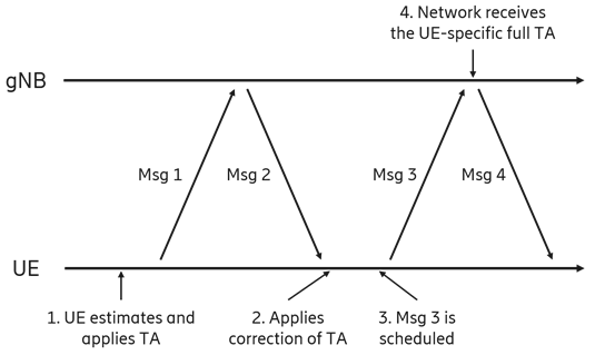
Read this one as a sequence of who knows the TA. At step 1 only the UE knows, and only approximately. At step 2 the network has measured the arrival of Msg1 and can send back a correction, but it still does not know the absolute value the UE started from. At step 3 the network has to schedule Msg3 while that ambiguity is still open, which is why it must assume the worst case delay in the cell. Only at step 4, once Msg3 has arrived, do both ends hold the same UE-specific TA. The whole point of the NTN additions is to make the gap between step 1 and step 4 as small and as cheap as possible.

<TR 38.821 - Figure 7.2.1.1.2-2: Framework on 2-step random access procedure for UE with location information >

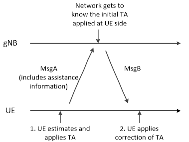
The 2-step version collapses that gap almost entirely. Because MsgA carries a PUSCH payload as well as a preamble, the UE can tell the network what advance it applied instead of leaving it to be inferred. The network therefore knows the UE-specific TA from the very first message and never has to schedule against a worst-case assumption. In a cell with 10 ms of differential delay that is not a small optimisation - it is the difference between scheduling for the cell and scheduling for the UE.

Worked Example : Where the 3GPP Numbers Come From

All the delay figures quoted in TR 38.821 come from one piece of geometry, and reproducing it is the quickest way to stop treating those numbers as magic. For a circular orbit of altitude h seen at elevation angle e from a point on the Earth's surface, the slant range is

d = sqrt( (R_e sin e)² + 2 R_e h + h² ) - R_e sin e

with R_e = 6,371 km, and the one-way propagation delay is d / c using c = 299,792,458 m/s (the exact value TR 38.821 states it used). Running that for the reference altitudes :

Every highlighted value is exactly what appears in the TR 38.821 reference tables - 1,932 km, 40,581 km, 12.89 / 25.77 ms, 238.74 / 270.73 ms and 477.48 / 541.46 ms. Three things fall out of this that are easy to miss when the numbers are just read off a table :

• The 'maximum' delays are all the 10� case. The minimum elevation angle is not a coverage parameter that happens to be in the table - it is what defines the worst-case delay, and therefore what every timing field range was sized against. Lower the minimum elevation and every number in this page moves.
• The transparent column is exactly twice the regenerative one, because the reference scenarios assume a feeder link of the same length as the worst-case service link. Real systems differ, which is why Common TA is signalled rather than derived.
• The spread within one LEO pass is enormous : 4.00 ms overhead versus 12.89 ms at the horizon, i.e. nearly 9 ms of variation on the same link with the same satellite. That is the number the UE's open-loop tracking has to follow continuously.

Field of view is not the same as a cell

That 9 ms figure is the spread across the satellite's entire field of view, and it is worth not confusing it with the 3.12 ms 'maximum differential delay within a cell' quoted in the reference table. A cell is one beam footprint - up to about 1,000 km for LEO - not the whole visible area, so the delay spread that a single cell's RACH design has to absorb is the smaller number. Both matter, but for different things : the field-of-view spread drives how fast the UE's open-loop estimate must track, while the within-cell spread drives the RACH and scheduling design.

Even that smaller number is brutal in radio terms. A normal cyclic prefix at 15 kHz subcarrier spacing is about 4.7 us. A 3.12 ms differential delay is therefore roughly 660 cyclic prefixes wide. There is no possibility of covering it with a margin or a guard interval - a per-UE timing advance is the only thing that can work, which is ultimately the reason GNSS is mandatory for an NTN UE.

Where the Numbers Live : SIB19 Parameters

Everything discussed on this page is signalled through SIB19 and its ntn-Config, so it is useful to have the mapping from concept to field in one place. The ASN.1 detail and the surrounding RRC structures are covered in NTN RRC (NR).

What Breaks When the Timing is Wrong

Timing faults in NTN rarely announce themselves as timing faults. They show up as a link that does not come up, or one that comes up and then quietly dies a minute later. The table below maps the common symptoms back to the mechanism responsible, which is usually the fastest way into a log.

3GPP Reference

• Non-Terrestrial Networks (NTN) - 3GPP Technology Article (2024)
• 3GPP TR 38.811 : Study on New Radio (NR) to support non-terrestrial networks
• 3GPP TR 38.821 :  Solutions for NR to support non-terrestrial networks (NTN)
• 3GPP TR 38.913 : Study on scenarios and requirements for next generation access technologies
• 3GPP TR 23.737 - Study on architecture aspects for using satellite access in 5G
• RP-193234 : Solutions for NR to support non-terrestrial networks (NTN)
• TS 22.261 : Service requirements for the 5G system; Stage 1 (Release 18)
• 3GPP TS 38.300 : NR and NG-RAN Overall Description - clause 16.14, the source of the timing relationship figure on this page
• 3GPP TS 38.213 : NR; Physical layer procedures for control - clause 4.2, the T_TA expression, K_offset and K_mac
• 3GPP TS 38.331 : NR; Radio Resource Control (RRC) protocol specification - SIB19, ntn-Config, TAInfo, EphemerisInfo
• 3GPP TS 38.321 : NR; Medium Access Control (MAC) protocol specification - Timing Advance Command MAC CE, HARQ feedback disabling
• 3GPP TS 38.211 : NR; Physical channels and modulation - the basic time unit T_c and cyclic prefix lengths
• 3GPP TS 38.101-5 : NR; UE radio transmission and reception; Part 5: Satellite access - UE frequency error and timing requirements over NTN
• 3GPP TR 36.763 : Study on NB-IoT / eMTC support for Non-Terrestrial Networks - the IoT-NTN counterpart of the timing work described here

Related Pages on this Site

• NTN Architecture - why a transparent payload doubles every number on this page
• NTN RACH - the preamble receiving window, overlapping RACH occasions, and the full 4-step / 2-step procedures
• NTN RRC (NR) - the SIB19 and ntn-Config ASN.1 behind every parameter listed above
• NTN Requirement - the delay and performance targets the timing design has to meet
• NTN Challenges - timing seen alongside the other NTN problems
• NTN Call Flow (NR) - the TA lifecycle as it appears in an actual log
• Web Simulator : 2D Satellite Orbit, Doppler, Distance and Elevation - vary the altitude, pass geometry and carrier and watch slant range, elevation and Doppler respond together
• Web Simulator : Doppler Effect and Propagation Delay - the underlying relationship on its own, without the orbital geometry

Other References

• Non-terrestrial networks (NTN) - R&S
• Non-Terrestrial Network Advantages, Challenges, and Applications - Keysight
• 5G & Non-Terrestrial Networks - 5G Americas White Paper (2022)
• Orbit of a satellite Calculator
• LEO Small-Satellite Constellations for 5G and Beyond-5G Communications
• Satellite Communications in the New Space Era: A Survey and Future Challenges
• Assessing satellite-terrestrial integration opportunities in the 5G environment  
• Satellite and Terrestrial Network for 5G
• Application of 5G new radio for satellite links with low peak-to-average power ratios
• 5G from Space: An Overview of 3GPP Non-Terrestrial Networks