RACH in NTN

The RACH process is a cornerstone of establishing connectivity in any wireless communication system, but its implementation in Non-Terrestrial Networks (NTN) brings a unique set of challenges. In case of terrestrial networks, signals travel relatively short and predictable paths, but NTN systems involve complex interactions influenced by the vast distances of satellite orbits, rapid mobility of spacecraft, and dynamic environmental conditions. These factors create various hurdles such as significant propagation delays, Doppler shifts due to satellite motion, and the challenges of maintaining synchronization across a broad and ever-changing coverage area. Additionally, the inherent constraints of satellite communication such as limited spectrum resources and increased contention among devices, further complicate the RACH process. Addressing these challenges requires innovative strategies and adaptations, making the optimization of RACH in NTN a critical area for advancing global connectivity.

• Potential Challenges in NTN RACH
• Challenges on Premable detection(4 Step RACH)
• Challenges on Rach Response Window
• Challenges on Contention Resoultion Timer
• 4 Step RACH Framework
• 2 Step RACH Framework
• The Two Branches : UE With and Without Location Information
• What Rel-17 Actually Specified
• What Breaks, and What it Looks Like

Why RACH is the Hardest Procedure to Port to NTN

Most NTN adaptations are about making an existing procedure tolerate a bigger number. RACH is different, and it is worth being clear about why before going through the individual challenges, because almost every item in the list below is a symptom of the same single problem.

The chicken and egg

Random access is the one procedure that has to work before the network knows anything about the UE. Every other uplink transmission in NR happens after the UE is already timing-aligned, because random access is what aligned it. In a terrestrial cell that bootstrap works because the delay is small enough that an uncompensated preamble still lands inside the receive window - the network measures the arrival time and tells the UE what to fix.

In NTN that bootstrap breaks. An uncompensated preamble from a GEO UE arrives hundreds of milliseconds late, long after the gNB has stopped listening. So the UE has to be timing-aligned before random access rather than as a result of it - which inverts the entire purpose of the procedure. That single inversion is what forces GNSS into the UE, ephemeris into the broadcast, and pre-compensation into the very first transmission.

NOTE : Keep this inversion in mind while reading the challenges below. Several of them - preamble detection ambiguity, response window sizing, contention resolution timing - look like separate problems but are all consequences of the same thing : the network can no longer assume that a message arrives roughly when it was sent, and can no longer measure the delay itself. The timing machinery that makes the pre-compensation possible is covered separately in NTN Timing Advance.

Potential Challenges in NTN RACH

Followings are various issues that may get involved in RACH Process in NTN environment. I think current 3GPP defines the specification only a small subset of these potential issues.

• Increased Latency and RTT
• Impact: The significant distance between the user equipment (UE) and the satellite leads to longer round-trip times (RTT), affecting the timing and responsiveness of the RACH process. This delay can cause timeouts and increase the time it takes for a UE to successfully complete the random access procedure.
• Considerations: RACH procedures and timers need adjustments to accommodate these longer delays.
• Timing Advance Challenges
• Impact: The dynamic nature of satellite orbits and their extensive coverage areas introduce complexities in accurately calculating and adjusting timing advance for user equipment (UE). Incorrect timing advance can lead to collisions between uplink transmissions from different UEs, or misalignment with the satellite's reception window, hindering successful communication.
• Consideration: To mitigate this, engineers are developing sophisticated algorithms that enable UEs to precisely estimate and dynamically adjust their timing advance, ensuring seamless synchronization with the satellite and minimizing the risk of transmission conflicts.
• Doppler Shift
• Impact: The relative movement between the satellite and the UE causes a Doppler shift in the frequency of the transmitted signals. This can affect the accuracy of frequency synchronization and potentially lead to unsuccessful RACH attempts.  
• Considerations: Robust frequency compensation techniques are crucial to mitigate the effects of Doppler shift.  
• Variable Channel Conditions
• Impact: Atmospheric effects, shadowing, and varying signal strengths due to the long distances can create unpredictable channel conditions. This can lead to higher error rates and make it difficult for the UE to reliably decode the random access responses from the satellite.  
• Considerations: Adaptive power control and robust coding schemes are essential to maintain reliable communication.
• Large Coverage Areas
• Impact: Satellites typically cover very large geographical areas, which can result in a higher number of UEs attempting random access simultaneously. This increases the likelihood of collisions and contention, potentially leading to multiple RACH attempts and delays.
• Considerations: Efficient RACH resource allocation and contention resolution mechanisms are needed to manage a large number of users.
• Collision Probability
• Impact: The inherent characteristic of satellites to cover vast geographical areas leads to a higher number of UEs contending for the same RACH resources. This increased contention elevates the probability of collisions between preambles transmitted by different UEs, reducing the efficiency of the RACH process and increasing latency in establishing network connections.
• Consideration: To optimize RACH efficiency, researchers are exploring various strategies, including advanced access control mechanisms, dynamic resource allocation, and contention resolution techniques, to minimize collisions and ensure timely access to the network.
• Synchronization Challenges
• Impact: Establishing initial synchronization with a non-terrestrial network can be challenging for UEs due to factors such as large frequency offsets caused by Doppler shift and timing errors arising from propagation delays. Failure to achieve accurate synchronization prevents UEs from successfully initiating the RACH process and establishing a connection.
• Consideration: Robust synchronization techniques are essential for enabling seamless connectivity. These techniques involve precise frequency estimation and compensation mechanisms, as well as accurate timing acquisition protocols, to ensure that UEs can effectively synchronize with the satellite network and initiate communication.
• Power Control Issues
• Impact: UEs within an NTN experience significant variations in path loss due to their diverse locations and distances from the orbiting satellite. Insufficient transmission power can result in the preamble failing to reach the satellite for detection, while excessive power can cause interference with other UEs, degrading overall network performance.
• Consideration: Adaptive power control mechanisms are crucial for optimizing signal strength. These mechanisms enable UEs to dynamically adjust their transmission power based on real-time channel conditions and their position relative to the satellite, ensuring reliable communication while minimizing interference
• Beam Management
• Impact: Satellites often use multiple beams to cover their service area. UEs might need to perform beam switching or acquisition, adding complexity to the RACH process.
• Considerations: Seamless beam handover and efficient beam tracking are important for maintaining connectivity during the RACH procedure.

Challenges on Premable detection(4 Step RACH)

In NTN, due to the varying distances between the User Equipment (UE) and the network, there can be a significant difference in the time it takes for a preamble to reach the network. There can be a few critical challenges due to this delay.

Issue 1 : Differential Delay Challenges

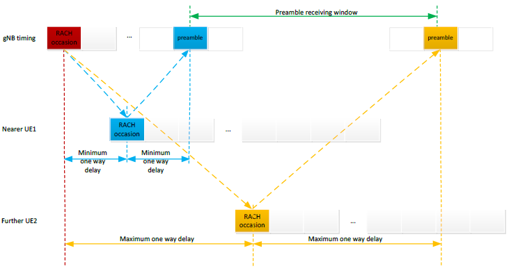
Due to the significant differences in propagation delays between UEs at varying distances from the base station, the preambles transmitted during a RACH occasion can arrive at different times. This differential delay complicates the network's ability to accurately receive and process these signals, leading to potential ambiguities in identifying the associated RACH occasions.

• Due to the vast distances in NTN cells, UEs within the same RACH occasion may transmit preambles that arrive at the network at different times.
• The diagram shows how the minimum and maximum one-way delays determine the timing of preamble arrivals.

<TR 38.821 - Figure 7.2.1.1.1.2-1: Preamble receiving window in NTN >

<TR 38.821 - Table 7.2.1.1.1.2-1: Maximum delay difference*2 for typical GEO and LEO cell >

Category	Typical Cell Size	Maximum Delay Difference * 2
GEO	1000 km	6.44 ms
	500 km	3.26 ms
LEO	200 km	LEO600: 1.306 ms LEO1200: 1.308 ms
	100 km	LEO600: 0.654 ms LEO1200: 0.654 ms

Reading those numbers : differential delay is really just the cell size

The four values in the table above look like they must have come out of a complicated orbital calculation. They did not, and there is a shortcut hiding in them that is worth extracting because it makes the whole PRACH dimensioning problem intuitive.

The worst case differential delay occurs when the cell sits at low elevation, near the edge of the satellite's field of view. At low elevation the line of sight is almost parallel to the ground, so a UE that is one cell-diameter further away across the ground is also almost exactly one cell-diameter further away in slant range. The delay difference therefore collapses to little more than the cell diameter divided by the speed of light :

maximum delay difference x 2  ≈  2 x ( cell diameter ) / c

The strongest evidence is already in the table

Look at the LEO row for a 200 km cell : 1.306 ms at 600 km altitude and 1.308 ms at 1200 km. The orbit altitude was doubled and the answer moved by 0.15 %. That is not a coincidence or a rounding artefact - it is the clearest possible demonstration that the differential delay is set by the cell size and essentially not by the orbit at all.

This gives a clean separation that is easy to carry around :

• Absolute delay is an altitude problem. GEO 541 ms versus LEO 26 ms - a factor of twenty. This is what breaks response windows, HARQ and every protocol timer.
• Differential delay is a cell size problem. A 1000 km cell has roughly 3.3 ms of spread whether it is fed from 600 km or from 35,786 km. This is what breaks preamble detection and forces the RACH occasion spacing.

The two are independent, and they are fixed by different mechanisms. Confusing them is the most common way to mis-dimension a PRACH configuration - which is exactly what the next section is about.

Issue 2: Overlapping RACH Occasions

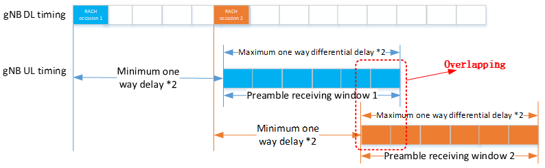
When RACH occasions are configured with inadequate time intervals between them, the preamble receiving windows for consecutive occasions may overlap. This overlap introduces a significant challenge, as it creates ambiguity for the network. In such cases, the network may find it difficult to determine which RACH occasion a received preamble belongs to, complicating the process of accurately calculating the timing advance required for synchronization. This issue can severely impact the efficiency and reliability of communication in Non-Terrestrial Networks.

• If the RACH occasions are configured with insufficient time gaps, the receiving windows for consecutive occasions might overlap.
• This can create ambiguity, as the network may struggle to associate a received preamble with its corresponding RACH occasion, making it difficult to calculate timing advance accurately.

<TR 38.821 - Figure 7.2.1.1.1.2-2: Ambiguity on preamble reception at the network side >

Possible Solutions

There are several potential solutions to address these issues as summarized below

• Proper PRACH Configuration: Extend the interval between consecutive RACH occasions so that the receiving windows do not overlap. The interval should be greater than twice the maximum one-way delay.
• Preamble Division: Assign preambles to specific groups linked to distinct RACH occasions to reduce confusion.
• Frequency Hopping: Use different frequency bands for preambles in overlapping occasions to distinguish between them.
• 2-Step RACH Assistance Information: Include identifiers like the SFN index in the messages to help the network link preambles to the correct RACH occasion.

<TR 38.821 - Table 7.2.1.1.1.2-2: Examples of feasible PRACH configurations for a typical GEO or LEO cell >

How that configuration table was actually derived

The PRACH configuration table above looks like a lookup that has to be taken on trust. It is not - the whole thing follows from one rule, and once you see the rule you can dimension a configuration for any cell size yourself.

The last column, ρ, is the number of PRACH opportunities per second, so 1/ρ is the spacing between consecutive RACH occasions. For the receiving windows not to overlap, that spacing simply has to be larger than the spread of arrival times, which is the 'maximum delay difference x 2' quantity from the earlier table. Lining the two tables up :

Every row is the same decision : take the arrival spread, and pick the next convenient PRACH periodicity above it. The PRACH Configuration Index column is then just whichever index in the TS 38.211 tables happens to produce that periodicity with the wanted preamble format - which is why several different indices appear for the same cell size.

NOTE : The quantity that sets the spacing is twice the maximum delay difference across the cell, not twice the maximum absolute one-way delay. The distinction is easy to gloss over and the two differ enormously : for GEO the absolute one-way delay is around 270 ms, which would imply RACH occasions roughly half a second apart and a ρ of about 2. What actually constrains the design is the 6.44 ms spread within the cell, and the table's ρ = 100 follows from that. This is the same absolute-versus-differential split described above - the absolute delay is dealt with by offsetting the windows and timers, not by spacing the RACH occasions.

The trade nobody escapes

Notice what the ρ column does as the cell grows : 1000 opportunities per second for a 100 km cell, down to 100 for a 1000 km cell. Spreading the RACH occasions further apart is the fix for the ambiguity problem, but it is a tenfold reduction in access opportunities - and a bigger cell also contains far more UEs. The two effects compound in the wrong direction.

That is the coupling between two of the challenges listed at the top of this page. Large coverage areas and collision probability are not independent of the differential delay problem - the standard cure for the third makes the first two worse. A large NTN cell therefore pays twice : more contenders, and fewer chances to contend. It is one of the strongest practical arguments for keeping NTN beam footprints small, quite apart from the link budget.

Why preamble format 3 keeps appearing

The preamble format column is worth a note of its own. Formats 0, 1 and 2 are long-sequence formats built on a 1.25 kHz subcarrier spacing, while format 3 uses 5 kHz. That four-fold increase in subcarrier spacing buys four times the tolerance to residual frequency error, which is precisely the currency NTN is short of - so format 3 turns up in a feasibility study for Doppler reasons rather than for any cell-size reason.

There is a deeper inversion here too. In a terrestrial network the preamble format is chosen mainly to make the cyclic prefix long enough to cover the round trip spread of the cell - which is what caps terrestrial cell radius at a few tens of kilometres. In NTN the UE pre-compensates its own delay before transmitting, so the CP no longer has to span the cell at all; it only has to absorb the residual error left after pre-compensation. That is the reason a 1000 km NTN cell can work with preamble formats that terrestrially would be limited to a small fraction of that radius, and it is another consequence of the bootstrap inversion described at the top of this page.

Challenges on Rach Response Window

In the Random Access (RA) procedure, a User Equipment (UE) sends a preamble (Msg1) to the base station and then monitors the Physical Downlink Control Channel (PDCCH) for a corresponding Random Access Response (Msg2). In terrestrial systems, this response is typically received within a short, predefined time window (ra-ResponseWindow) of just a few milliseconds. However, in NTN, the propagation delays are much longer due to the large distances involved (e.g., communication with satellites in Geostationary Earth Orbit (GEO) or Low Earth Orbit (LEO)). This extended delay means that the RAR cannot be received within the terrestrial time window, resulting in failed RA attempts and the need for procedural enhancements.

Simply put,

• When a device wants to connect, it sends a "preamble" (Msg1) – think of it like knocking on a door.
• It then waits for a "response" (Msg2) – like someone opening the door.
• This waiting time is the "response window".
• Normally, this works fine because the signal doesn't travel very far.
• But with satellites, the signal has to travel a huge distance, causing a delay. The response might come after the device has stopped waiting, causing connection problems.

<TR 38.821 - Figure 7.2.1.1.1.2-3: RAR window in NTN >

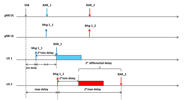
The maximum differential delay varies by orbit type:

• GEO: 10.3 ms, requiring a response window extension of at least 20.6 ms (2 × maximum differential delay), which exceeds the default 10 ms window.
• LEO: 3.18 ms, requiring a response window extension of 6.36 ms, which is within the 10 ms default but still necessitates careful configuration.

For UEs initiating RA from locations with significantly different propagation delays (e.g., cell edges), a response window that does not consider these delays risks missing the RAR altogether.

Possible Solutions

To address this challenge, two main adjustments to the ra-ResponseWindow are proposed:

• Configurable Offset for the Start of the Response Window:
• The start of the RAR window should include an offset to account for the propagation delay in NTN. This offset should be configurable to adapt to varying network scenarios.
• For UEs with location information, the offset can be calculated using the known round-trip delay, which eliminates the need to extend the response window further.
• Extension of the Response Window Duration:
• For UEs without location information, where the round-trip delay cannot be accurately estimated, the window itself must be extended to ensure the RAR is received within the valid monitoring duration.
• The extended duration must accommodate the maximum differential delay (i.e., the time difference between the minimum and maximum propagation delays within a cell), plus an additional margin for processing delays at the gNB and scheduling flexibility.

Challenges on Contention Resoultion Timer

During the random access procedure in cellular networks, after the User Equipment (UE) sends an RRC Connection Request (Msg3), it waits for Msg4, the contention resolution message, to determine if its random access attempt was successful. The duration for which the UE monitors for Msg4 is governed by the ra-ContentionResolutionTimer. This timer starts immediately after Msg3 is transmitted.

In NTN scenarios, due to the long distances between the UE and the base station (e.g., satellite communication in GEO or LEO), the round-trip delay is much longer compared to terrestrial systems. While the maximum configurable value of the ra-ContentionResolutionTimer can technically cover these longer delays, this approach is inefficient and may unnecessarily consume power on the UE side. NTNs often require power-efficient operation, especially for UEs in remote or battery-constrained applications. Therefore, the default behavior of the ra-ContentionResolutionTimer must be adjusted to better align with NTN propagation delays while conserving UE power.

Possible Solutions

A possible solution is to introduce an offset for the start of the ra-ContentionResolutionTimer in NTN scenarios. Instead of starting the timer immediately after Msg3 transmission, the timer would begin only after an offset period that accounts for the expected round-trip delay in NTN.

This adjustment ensures the timer is active only during the period when Msg4 is expected to be received. By aligning the timer with the NTN-specific delays, the UE avoids unnecessarily monitoring for Msg4 during periods when it is unlikely to arrive. This saves power while still ensuring compatibility with NTN's longer delays.

NOTE : Benefits of the Offset-Based Timer Adjustment:

• Power Efficiency: The UE will only monitor for Msg4 when it is realistic for the message to arrive, reducing unnecessary power consumption.
• Flexibility for Various Orbits: The offset can be configured based on the type of NTN, whether GEO or LEO, as the propagation delay varies significantly between these systems.
• Scalability: This approach accommodates NTNs of different sizes and propagation delay characteristics without requiring extensive modifications to the standard contention resolution procedure.
• Robustness: Aligning the timer with realistic delays prevents premature expiration of the contention resolution timer, which could otherwise cause unnecessary retransmissions or failures in NTN communication.

4 Step RACH Framework

Accurate timing is crucial in NTN, and this 4-step process ensures that devices and the network can establish a common understanding of time despite the vast distances and dynamic conditions. It's a bit like a cosmic dance, where precise timing ensures a harmonious connection across the vastness of space.

<TR 38.821 - Figure 7.2.1.1.1.2-9: Framework on 4-step random access procedure for UE with location information >  

Step 1. Initial Timing Advance Estimation / UE Timing Advance Estimation and Application

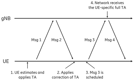
Before a device (UE) even begins to transmit its "hello" message (Msg1), it needs to figure out how long it will take that message to reach the satellite. This is like calculating the travel time for a postcard sent across continents.

• Regenerative Architecture: If the satellite processes the signal directly, the UE needs to know the satellite's position. This can be obtained from publicly available satellite data (like an ephemeris) or broadcast by the satellite itself. It's like checking a map to see how far away your destination is.
• Transparent Architecture: Things get trickier if the signal is routed through a ground station. Now, the UE needs to factor in both the distance to the satellite and the distance from the satellite to the ground station. This might involve the satellite broadcasting its position and the ground station's location, or providing information about the link between them. It's like calculating a multi-stop journey with connecting flights.

Step 2. Timing Advance Correction / Timing Advance Correction via Msg2

Once the network receives Msg1, it responds with a Random Access Response (RAR) in Msg2, which includes a timing advance correction. This correction accounts for the UE’s estimation errors in Step 1, fine-tuning the alignment.

Once the UE receives a response (Msg2) acknowledging its initial message, it refines its timing estimate. This is because its initial guess might have been slightly off, like arriving a bit early or late for an appointment. The UE adjusts its timing based on the feedback from the network, ensuring its subsequent messages are perfectly synchronized.

Step 3. Scheduling with Uncertainty / Scheduling of Msg3

The network now needs to schedule the UE's next transmission (Msg3), but it doesn't yet know the exact timing advance the UE is using. To avoid conflicts, the network plays it safe by assuming the maximum possible delay. This is like booking a meeting room for a longer duration to accommodate potential delays.

In other words, the network schedules Msg3 (RACH response message) without yet having an absolute value of the UE’s specific timing advance. To handle this, the network must use a conservative approach, such as:

• Allocating resources based on the maximum propagation delay in the satellite’s coverage area.
• Accounting for the maximum differential delay within the satellite cell.

These strategies ensure Msg3 reaches the gNB reliably, even under the worst-case timing misalignment scenarios.

Step 4. Final Synchronization

Finally, when the network receives Msg3, it learns the precise timing advance of the UE. Both sides are now perfectly in sync, like two dancers flawlessly coordinated in their movements. This ensures smooth and efficient communication from this point onward.

When the UE sends Msg3, the network finally receives and calculates the exact timing advance specific to the UE. At this stage, both the UE and the network are synchronized with a precise TA value, which is critical for the subsequent exchange of data.

In cases where the UE has location information, it can optimize the process by compensating for a specific TA during Msg1. This specific TA is determined using the difference between the UE’s estimated delay and a reference point (d1 - d0). Meanwhile, the network compensates for a "common TA," defined by the distance between a reference point and the gNB.

2 Step RACH Framework

The 2-step RACH process significantly reduces the time it takes to establish a connection. By including assistance information in the initial message, the UE helps the network quickly understand its timing needs. This leads to faster and more efficient communication, which is particularly valuable in the dynamic environment of NTN, where delays can be significant. It's like having a more direct conversation, cutting through the noise and getting connected quicker.

Overall, the 2-step RACH procedure offers a robust framework for managing timing advance in NTN, leveraging efficient message design and feedback mechanisms to overcome the unique challenges of satellite communication. This approach not only simplifies the RACH process but also enhances its reliability, paving the way for more effective satellite-based 5G deployments.

<TR 38.821 - Figure 7.2.1.1.2-2: Framework on 2-step random access procedure for UE with location information >  

Step 1.  Initial Timing Advance and Assistance Information/UE Timing Advance Estimation and Transmission of MsgA

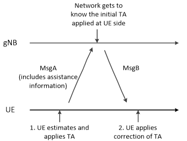
In this streamlined process, the device (UE) still needs to estimate the initial timing advance before sending its first message (MsgA). However, there's a clever twist.  Along with its "hello" message, the UE also includes extra information – a hint, if you will – about its estimated timing advance. This gives the network a head start in understanding the UE's position and timing. It's like including your location in a message so the recipient knows how long it took to arrive.

Putting it in more detail, the process begins with the UE estimating and applying an initial timing advance before sending MsgA. MsgA serves a dual purpose—it includes a preamble transmitted on the PRACH and a payload transmitted on the PUSCH. This payload contains critical assistance information that allows the network to determine the initial timing advance applied by the UE.

This step provides a significant advantage over the 4-step RACH procedure, as the network now has direct access to the UE's timing advance information from the first message. This eliminates the need for the network to rely solely on assumptions or maximum propagation delay estimates when scheduling subsequent transmissions. The inclusion of assistance information in MsgA simplifies the synchronization process, making it particularly suitable for NTN environments with long and variable delays.

Step 2.  Contention Resolution and Final Adjustment/Contention Resolution and Timing Advance Correction via MsgB

Following the transmission of MsgA, the UE monitors the network for a response within a configured window. If contention resolution is successful, the network responds with MsgB, which completes the RACH procedure. At this stage, the UE applies any necessary timing advance corrections based on the feedback received in MsgB.

By the end of this step, both the UE and the network have a precise understanding of the UE-specific timing advance. This mutual awareness ensures that subsequent communication is tightly synchronized, even in the face of the high latency and dynamic conditions inherent to NTN.

NOTE : What are Benefits of the 2-Step Procedure in NTN ?

The primary benefit of this approach lies in its ability to streamline the RACH process while addressing key challenges of NTN environments:

• Improved Timing Accuracy: The inclusion of timing advance information in MsgA allows the network to avoid relying on maximum delay estimates, reducing resource inefficiency and improving scheduling precision.
• Reduced Complexity: By consolidating operations into two steps, this procedure minimizes the overhead associated with the additional steps in the 4-step process.
• Adaptation to NTN Dynamics: The reduced latency and quicker resolution make the 2-step RACH better suited for NTN scenarios, where long delays and high mobility of satellites complicate synchronization.

The Two Branches : UE With and Without Location Information

Both of the framework figures above carry the same qualifier in their captions, and it is easy to read past : 'for UE with location information'. That phrase is not decoration. TR 38.821 deliberately studied two parallel branches throughout, and which one you assume changes almost every design decision on this page.

Reading the challenge sections above again with this split in mind is instructive. Nearly all of the 'possible solutions' listed - extending the response window, partitioning preambles between occasions, hopping frequency between occasions, adding an SFN index to the assistance information - exist to make the left-hand column workable. They are the price of not knowing where the UE is.

What Rel-17 Actually Specified

Everything on this page up to here comes from TR 38.821, which is a study document - it explores the problem space and lists candidate solutions without committing to any of them. It is worth knowing which candidates actually became specification, because 3GPP resolved the two-branch question in the simplest possible way.

Rel-17 closed the left-hand branch entirely

A Rel-17 NR-NTN UE is required to have GNSS capability, and is required to hold a valid position fix together with valid ephemeris and Common TA from SIB19 before it may access the cell at all. There is no 'UE without location information' in the normative design. That one decision retires most of the problems on this page rather than solving them : if every UE pre-compensates its own delay before transmitting, then preambles from the cell centre and from the cell edge arrive at essentially the same time, and the differential delay never reaches the receiver in the first place.

< 38.300 - Figure 16.14.2.1-1: Illustration of timing relationship (for collocated gNB and NTN Gateway) >

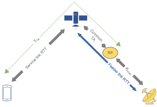
The reference point (RP) in this figure is what the pre-compensation is aimed at. Every UE in the cell advances its transmission so that its signal is aligned at the RP rather than at its own antenna - which is why their preambles converge instead of spreading out. The UE computes the service link part itself from GNSS and ephemeris; the network broadcasts the rest as Common TA. The full machinery is covered in NTN Timing Advance.

NOTE : This is a good illustration of how a 3GPP study relates to the specification that follows it. TR 38.821 is not a list of things that were built - it is the record of a search, and a large part of its value is showing which problems disappeared once one architectural decision was made. The mandatory-GNSS decision is the single hinge on which most of this page turns.

What Breaks, and What it Looks Like

NTN RACH problems rarely present as 'random access failed'. They present as a UE that attaches in one place and not another, or at one time of day and not another. The table below maps the common patterns back to the mechanism.

NOTE : The elevation-dependent row is worth dwelling on, because it produces the most confusing field reports. Since differential delay is worst at low elevation, a marginal PRACH configuration fails in a band around the horizon and works fine in the middle of the pass - so the same UE in the same location succeeds and fails on a cycle set by the satellite's orbit rather than by anything the user did. The pass profile plots on the NTN Timing Advance page show why the geometry at the start and end of a pass is so different from the middle.

Related Pages on this Site

• NTN Timing Advance - the pre-compensation machinery that makes NTN RACH possible, and where K_offset comes from
• NTN RRC (NR) - SIB19, ephemeris, ta-Common and the RACH-related NTN parameters
• NTN Architecture - why a transparent payload doubles the delay the RACH design has to absorb
• NTN Call Flow (NR) - the random access procedure in a real message sequence
• NTN Challenges - RACH seen alongside the other NTN problems
• Web Simulator : 2D Satellite Orbit, Doppler, Distance and Elevation - watch how the slant range and its spread change through a pass

3GPP Reference

• Non-Terrestrial Networks (NTN) - 3GPP Technology Article (2024)
• 3GPP TR 38.811 : Study on New Radio (NR) to support non-terrestrial networks
• 3GPP TR 38.821 :  Solutions for NR to support non-terrestrial networks (NTN)
• 3GPP TR 38.913 : Study on scenarios and requirements for next generation access technologies
• 3GPP TR 23.737 - Study on architecture aspects for using satellite access in 5G
• RP-193234 : Solutions for NR to support non-terrestrial networks (NTN)
• TS 22.261 : Service requirements for the 5G system; Stage 1 (Release 18)
• 3GPP TS 38.211 : NR; Physical channels and modulation - PRACH preamble formats, sequence lengths and the PRACH configuration tables
• 3GPP TS 38.213 : NR; Physical layer procedures for control - clause 4.2 for the NTN timing relationships, and the random access procedure clause
• 3GPP TS 38.321 : NR; Medium Access Control (MAC) protocol specification - ra-ResponseWindow, msgB-ResponseWindow and ra-ContentionResolutionTimer, including the NTN start offsets
• 3GPP TS 38.331 : NR; Radio Resource Control (RRC) protocol specification - SIB19, ntn-Config, RACH-ConfigCommon and ta-Report
• 3GPP TS 38.300 : NR and NG-RAN Overall Description - clause 16.14, the NTN timing relationship figure used above
• 3GPP TR 36.763 : Study on NB-IoT / eMTC support for Non-Terrestrial Networks - the IoT-NTN counterpart, where the RACH constraints are tighter still

Other References

• Non-terrestrial networks (NTN) - R&S
• Non-Terrestrial Network Advantages, Challenges, and Applications - Keysight
• 5G & Non-Terrestrial Networks - 5G Americas White Paper (2022)
• Orbit of a satellite Calculator
• LEO Small-Satellite Constellations for 5G and Beyond-5G Communications
• Satellite Communications in the New Space Era: A Survey and Future Challenges
• Assessing satellite-terrestrial integration opportunities in the 5G environment  
• Satellite and Terrestrial Network for 5G
• Application of 5G new radio for satellite links with low peak-to-average power ratios
• 5G from Space: An Overview of 3GPP Non-Terrestrial Networks