RE Map to Antenna / Antenna to RE Map

This is basically for OFDM/SC-FDM at high level. But I tried to describe this in such as way that is helpful for you to program this process (Actually this is based on my experience of coding this part in matlab). However, I will not write on this procedure in full details with each specific numbers and data since it is too much for the single page. For further details, I will put the link to various different pages which would give you a specific examples and details.

The page follows one idea in four directions. The RE Map is a grid of complex values, one per subcarrier and symbol. The transmitter has to turn that grid into a waveform at the antenna, and the receiver has to turn the waveform back into the grid. The downlink does it with OFDM and the uplink with SC-FDMA, and the difference between the two sits in one extra transform.

Downlink : RE Map to Antenna

In this section, I will describe the process highligted as shown below. May look simple single step, but it is pretty complicated process and confusing.. it would be very hard in very detail unless you try to program (code) this process.

In this page, I will describe the process in the unit of a slot. If you think you understand overall logics explained here, refer to the example in OFDM page (the example in the page is for WLAN, not for LTE.. but overall logic is almost same). If you want LTE specific example for this process, refer to following two pages.

The drawing below is the downlink transmitter chain of 36.211, from scrambling to OFDM signal generation, with the clause number under each block. The highlighted box at the right is the part this section covers. The two arrows below it show its input, a resource grid of one slot, and its output, a time domain signal with a cyclic prefix in front of each symbol.

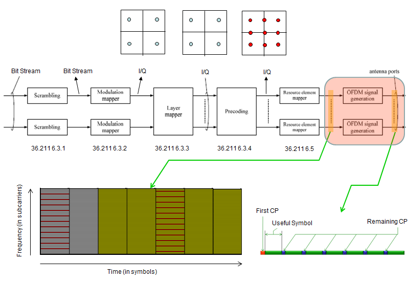
The 36.211 downlink chain from scrambling through modulation mapper, layer mapper, precoding and resource element mapper to OFDM signal generation, with the OFDM signal generation block highlighted and linked to a one slot resource grid and to a time signal with a first CP, useful symbols and remaining CPs

The RE Map is the input of OFDM signal generation. Everything on this page happens inside that one block.

Each block carries its clause : 36.211 6.3.1 for scrambling up to 6.3.4 for precoding, and 6.5 under the resource element mapper.
The grid has seven columns : one slot of normal CP, with time running to the right and frequency running up.
The first CP is drawn in a different colour : it is longer than the remaining ones, which the numbers below explain.

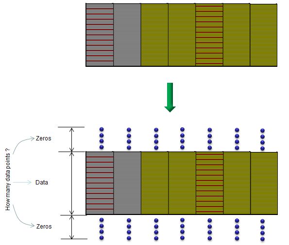
Adding Zero Pads : After you get the resource element map with all the data filled in, add a trails of zeros (Zero Pad) on both sides of each column (OFDM Symbol) of the resource map as shown below. Now your question would be, how many zeros I need to add ? What would be the number of data points for each section ?. The answer is different depending on System Bandwidth. For this, refer to page : Physical Layer Parameters - FDD, Downlink

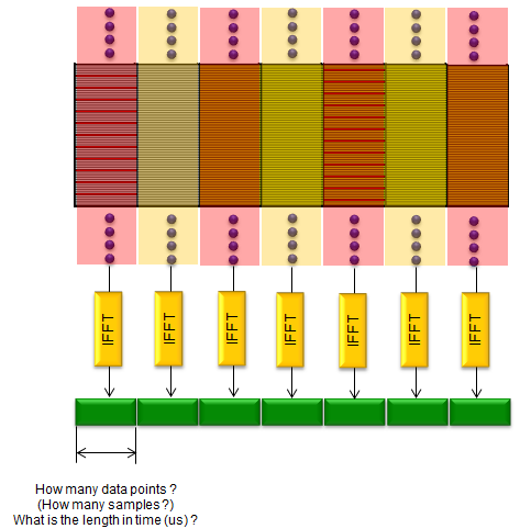
A one slot resource grid before and after zero padding, with zeros added above and below the data in every column and the question how many data points

Doing IFFT: Do IFFT for each OFDM Symbol and you will get the time domain data for each of OFDM Symbol. What would be the number of data points in each of the time domain OFDM Symbol ? The answer is different depending on System Bandwidth. For this, refer to page : Physical Layer Parameters - FDD, Downlink

Each zero padded column going through its own IFFT block and becoming one time domain symbol, with the questions how many samples and what is the length in time

Adding Cyclic Prefix : Now add Cyclick Prefix for each of the symbol. How many samples in each of the cyclic prefix ? The answer gets different whether it is the first symbol or non-first symbol and depends on the system bandwidth. For this, refer to page : Physical Layer Parameters - FDD, Downlink

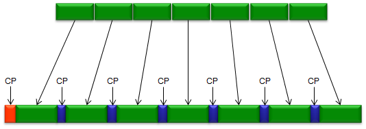
Seven time domain symbols each receiving a CP in front, with the first CP drawn in red and the other six in blue

D/A Converter/Up Converter : The last step is to convert the symbol data to analog and unconvert it to the carrier frequency and transmitted to Antenna. I think I oversimplified this step and this step would required complicated/sophisticated hardware design, but this is out of the scope of this page.

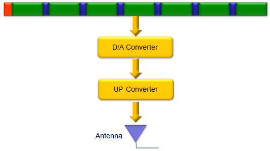
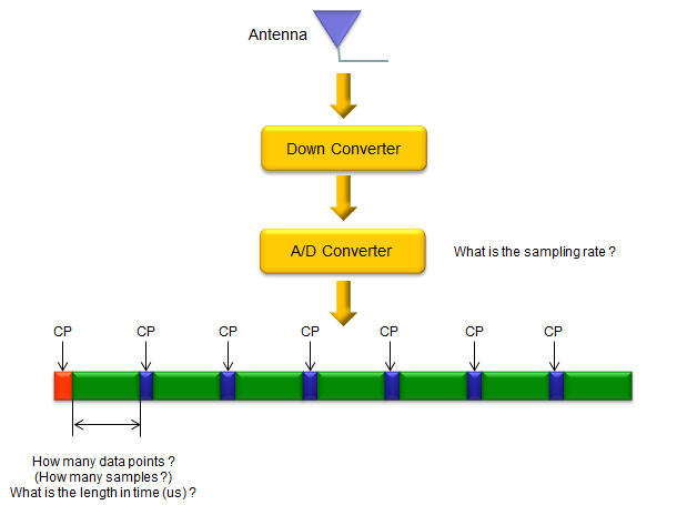
The slot of time samples going through a D/A converter and an up converter to the antenna

Now let's answer the questions the drawings ask, using 20 MHz as the example. 36.211 clause 6.12 defines the OFDM signal with N = 2048 for 15 kHz subcarrier spacing. So one IFFT has 2048 inputs, and the sampling rate is 2048 x 15 kHz, which is 30.72 MHz.

At 20 MHz there are 100 RBs, which is 1200 subcarriers. In the downlink the DC input of the IFFT stays empty, so 600 subcarriers go below it and 600 above it. The remaining 847 inputs are the zero pads, split between the two edges.

The cyclic prefix is counted in the same samples. With normal CP, 36.211 Table 6.12-1 gives 160 samples to symbol 0 of each slot and 144 samples to symbols 1 to 6. One slot is therefore 7 x 2048 + 160 + 6 x 144 = 15360 samples, which is exactly 0.5 ms at 30.72 MHz. The longer first CP is what makes the seven symbols fill the slot without a remainder.

The specification only writes the 2048 point version. A narrower bandwidth can use a smaller IFFT, for example 1024 points at 10 MHz with 15.36 MHz sampling. The CP lengths then scale down by the same factor, to 80 and 72 samples. That is an implementation choice rather than a separate rule, and the page linked above lists the usual values per bandwidth.

One IFFT per OFDM symbol : at 20 MHz it has 2048 inputs, 1200 with data and the rest zero.
The DC subcarrier is not used in the downlink : the RE Map is split into two halves around it.
160 and 144 : the first CP of a slot is 160 samples and the others are 144, at 30.72 MHz with normal CP.
15360 samples per slot : the numbers add up to exactly 0.5 ms.

Downlink : Antenna to RE Map

This is about receiving the OFDMA signal and demodulate it and construct RE Map from the demodulated bit stream. In reality, demodulation process is much more complicated than the modulation because you would require a lot of channel estimation and compenstion (Equalization), and finding synchronization. However, I assume that we are in a ideal channel and no need for this kind of compensation or synchronization. Once you understand the overall logic of this process, try your understanding with a real example : LTE DL(OFDM) Demodulation.

The receiver runs the transmitter chain backwards, and every number from the section above comes back. The drawings below follow the same order: sample the signal, cut off the CPs, take the FFT, and throw away the edges.

Down convert and Sampling (A/D Converter) : The first step is to downconvert the signal received by the antenna, downconvert it and sample it with A/D Converter. Assuming that everything is under ideal condition, the most important this to determined the proper sampling rate. Ideally, you can set any sampling rate as far as it is above the Nyquist Criterial, but it would help a lot in following steps if you sample it as specified in Physical Layer Parameters - FDD, Downlink

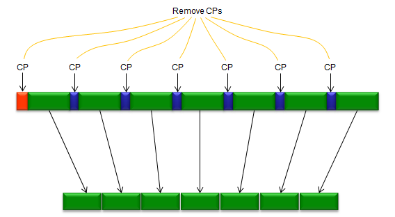
The antenna feeding a down converter and an A/D converter with the question what is the sampling rate, producing a slot of symbols with a CP marked before each one

Remove CP (Cyclic Prefix) : Now you have the time domain signal and the next step is to remove the Cyclic Prefix. To do this, you have to know exactly what is the number of samples in each symbol and how many samples are assigned for the Cyclic prefix. It depends on the system bandwidth and refer to Physical Layer Parameters - FDD, Downlink for the details.

The seven CPs of a slot being removed, leaving seven useful symbols

Do FFT : Next step is to do FFT for each OFDMA Symbol as shown below. Note that the result of this FFT will include the frequency area which is out side of the resource map. As in other steps, it is important to know how many samples (data points) you will get in the result of FFT and you can get the detailed information on this from Physical Layer Parameters - FDD, Downlink

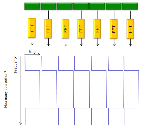
Each useful symbol going through its own FFT, giving a magnitude against frequency trace that is high in the middle and low at both edges

Remove the Rejection Area and Map to RE Map : The last step is relatively simple. Just remove the data points which is outside of the sub carriers of the system bandwidth and fill out the resource map with the remaining data. The important things is to cut out the exact data points.

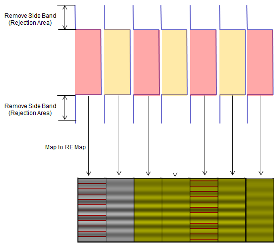
The FFT output of each symbol with the side bands at the top and bottom marked as rejection area, and the remaining middle part mapped into a one slot RE map

The receiver ends with the same one slot grid the transmitter started from. Only the order of the steps is reversed.

The FFT output is wider than the grid : the flat low parts at the top and bottom of each trace are the zero pads the transmitter added.
The side bands are the rejection area : they are cut off before the data goes back into the RE Map.
Seven columns in, seven columns out : the grid at the bottom matches the one at the start of the downlink section.

Two details make the exact cut harder than it looks. The first is the CP length. The receiver removes 160 samples before symbol 0 and 144 before each of the others, and a one sample error adds a phase ramp across the subcarriers of that symbol. The second is the DC bin. The FFT output has one bin at DC that carries nothing in the downlink, so the 600 lower and 600 upper subcarriers must be taken from either side of it.

The receiver needs the same numbers : FFT size, CP lengths and the position of the DC bin all come from the transmitter side.
Skip the DC bin : it sits between the two halves of the grid and holds no data.
Channel estimation is left out here : a real receiver equalizes the grid with the reference signals before it reads any data.

Uplink : RE Map to Antenna

In case of Uplink, the term 'RE Map' may mislead or confuse you a lot. Because most of us (including me) are more familiar with downlink frame structure and RE Map than the Uplink, when you talk about 'one resource element', you may easily associate it with 'one 15 Khz subcarrier', but in uplink you should not correlate the one resource element into 15 Khz subcarrier. As in the downlink case, RE Map refers to the signal structure at the output of [Resource Element Mapper] as shown below. In case of downlink, the data represented in (A) is almost directly trasnsfered to the corresponding to resource element in RE Map (assuming that this is single antenna configuration). and if you take out a data from all the resource elements from RE map and plot it onto a complex plane, you would see a distict constellation, but in case of uplink you would not see such a distict constellation if you take out all the data from resource Map and plot it because the data in each of the resource elements are the result of FFT of the original modulation data. The constellation would be something as in (D). If you want to get the distict constellation from the data in the UL RE Map, you have to do IFFT (you can see an example in Matlab :ToolBox : LTE : Uplink : PUSCH ).

The drawing below is the uplink chain of 36.211 with labels (A) to (G) on the signal at each stage. The key block is the transform precoder between the layer mapper and precoding, which the downlink chain does not have.

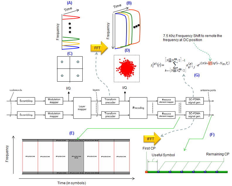
The 36.211 uplink chain with a transform precoder, labelled A for the modulation symbols, B for their FFT, C for a clean QPSK constellation, D for a noise like cloud from the RE map, E for the PUSCH and PUCCH resource grid, F for the time signal with CPs and G for the SC-FDMA formula with the half subcarrier shift

In the uplink the RE Map holds the FFT of the modulation symbols, so the values in it no longer look like a constellation.

(A) and (C) are before the transform precoder : these are ordinary modulation symbols, and they form the clean constellation in (C).
(B) and (D) are after it : the FFT spreads each symbol over all the allocated subcarriers, and the plot in (D) is a cloud.
(E) is the uplink grid : PUSCH in the middle, PUCCH at both edges, and the PUSCH RS in the middle symbol of the slot.
(G) marks the 7.5 kHz shift : the term k + 1/2 in the SC-FDMA formula moves every subcarrier by half a subcarrier.

If you are interesting in implementing this process in your code (matlab, C etc), I think following illustration would be more helpful. For simplicity, I assumed the case of single antenna (SISO) so that we don't have to care about layer mapping, precoding. Also, I illustrated the case of processing only one symbol. Note that this process applies only for PUSCH. PUSCH-DMRS is a little bit different. Actually, PUSCH-DMRS process is a little bit simpler because it does not go through Transform Precoder.

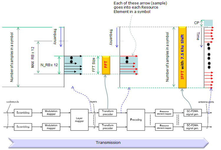
Uplink transmission of one symbol: N_RB x 12 modulation symbols go through an FFT of the same size, are placed on N_RB x 12 of the MAX RB x 12 subcarriers, and go through an IFFT with a 7.5 kHz shift before the CP is added

Two transforms in a row. A small FFT over the allocated subcarriers, then the full size IFFT over the whole bandwidth.

The FFT size is N_RB x 12 : it matches the allocation of this UE, not the system bandwidth.
Each FFT output goes to one resource element : the callout at the top says so, and the outputs sit inside the MAX RB x 12 range.
The IFFT covers the number of samples in a symbol : it is the same size as in the downlink, and it carries the 7.5 kHz shift.

The transform precoder has a size rule of its own. 36.211 clause 5.3.3 sets its length to 12 times the number of PUSCH RBs. It also requires that number of RBs to be a product of powers of 2, 3 and 5. So a UE can get 24 or 25 RBs, but not 7, 11 or 13, because those numbers have another prime factor.

The half subcarrier shift changes the DC handling too. The downlink leaves the DC subcarrier empty. The uplink cannot do that, because the transform precoder output has to stay on contiguous subcarriers. Instead, 36.211 clause 5.6 shifts every subcarrier by 7.5 kHz, so no subcarrier sits exactly on DC.

The uplink RE Map is not a constellation : it holds the DFT of the modulation symbols.
The allocation must be 2, 3 and 5 smooth : the number of PUSCH RBs is a product of powers of 2, 3 and 5.
No empty DC subcarrier in the uplink : the 7.5 kHz shift takes its place.
DMRS skips the transform precoder : it is generated directly in the frequency domain.

Uplink : Antenna to RE Map

This is about receiving the SC-FDMA signal and demodulate it and construct I/Q Constellation (Actually one step further than RE Map) from the demodulated bit stream. In reality, demodulation process is much more complicated than the modulation because you would require a lot of channel estimation and compenstion (Equalization), and finding synchronization. However, I assume that we are in a ideal channel and no need for this kind of compensation or synchronization. Once you understand the overall logic of this process, try your understanding with a real example : LTE UL(SC-FDM) Demodulation.

Uplink reception of one symbol: after the CP is removed, an FFT with a 7.5 kHz shift gives all subcarriers, only the allocated N_RB x 12 part is cut out, and an IFFT of that size gives back the modulation symbols

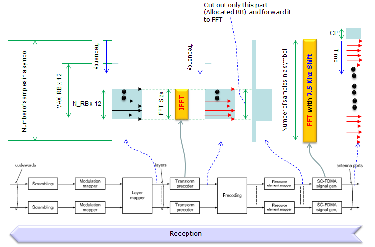
The receiver undoes the two transforms in reverse order. The full size FFT comes first, and the small IFFT over the allocated RBs comes last.

The FFT carries the 7.5 kHz shift too : the receiver removes the same half subcarrier offset the transmitter added.
Only the allocated RBs are cut out : the callout at the top points at the N_RB x 12 part that goes on to the IFFT.
The IFFT size is N_RB x 12 : it inverts the transform precoder and gives the constellation back.

The receiver has to know the allocation before it can take the second step. The eNB knows it because it sent the grant, so the size and the position of the cut are never guessed. An equalizer normally sits between the cut and the IFFT, because the channel is estimated per subcarrier from the DMRS.

Two transforms back : a full size FFT, then an IFFT the size of the allocation.
The grant defines the cut : the eNB uses the RBs it granted to find the part of the spectrum to keep.
Equalization comes before the small IFFT : the DMRS gives the channel per subcarrier, so it is corrected in the frequency domain.

Reference

Every step on this page is defined in one specification. The downlink signal generation is in clause 6.12 and the uplink one in clause 5.6.

[1] 36.211 : 3GPP - E-UTRA; Physical channels and modulation, v19.3.0. Clause 5.3.3 transform precoding, clause 5.6 SC-FDMA baseband signal generation, clauses 6.3 to 6.5 the downlink chain, and clause 6.12 with Table 6.12-1 OFDM baseband signal generation.