In this posts, I will show you the process to convert the frequency domain OFDM Symbol into time doing data which is transmitted by the antenna. This posts would show you the all the process from the beginning to the end of Downlink process.

Every channel on the previous pages lives in the resource grid, which is a frequency domain object. The antenna needs a sequence of time domain samples instead. The step between the two is OFDM modulation: an IFFT per OFDM symbol and a cyclic prefix in front of each one.

Followings are the topics to be covered in this page.

• SISO - Generating Time Domain Data
• Plotting Time Domain Data for Each OFDM Symbol
• Plotting Resource Grid and Time Domain for whole Radio Frame
• Plotting Frequency Spectrum
• Reference

SISO - Generating Time Domain Data

How does a resource grid become a waveform? This section builds the grid of all ten subframes of one radio frame with one antenna, and passes the whole frame to lteOFDMModulate. The later sections take the resulting samples apart again.

% First you have to define properites of a eNodeB.  

% NDLRB indicate System Bandwith in the unit of RBs.

% NDLRB 6 = 1.4 Mhz, NDLRB 15 = 3.0 Mhz, NDLRB 25 = 5.0 Mhz,

% NDLRB 50 = 10 Mhz, NDLRB 75 = 15 Mhz, NDLRB 100 = 20 Mhz

% CellRefP indicate number of downlink Antenna. CellRefP = 1 means 1 transmission antenna (SISO)

% NCellID indicate PCI (Physical Cell Identity) of the Cell

% NSubframe indicate the subframe number.

 

% In this example, most of these parameters are kept same for all subframe, but NSubframe value will be

% changed. so NSubframe will be set within the for loop.

 

enb.CyclicPrefix = 'Normal';

enb.PHICHDuration = 'Normal';

enb.Ng = 'Sixth';

enb.NDLRB = 6;

enb.CellRefP = 1;

enb.DuplexMode = 'FDD';

enb.NFrame = 0;

enb.NCellID = 0;

enb.CFI = 1;

 

% Now I will create an array variabel that will store all the subframe. It is initiailized with the empty array.

 

txFrameGrid = [];

 

% Now I will create a simple for loop and within the for loop I put the routine for creating all the signal and

% channel creation routing for each subframe. I just copied the whole routine from PDSCH creation example.

 

for subframeNo = 0:9   % start of for loop

 

% As I said, the enb paramters that does not change for each subframe is placed out side of the for loop

% I only put the chaning parameter (NSubframe) in this example within the forloop and associate it with

% for loop counter. Of course, which parameter you want to change for each subframe is up to you.

 

enb.NSubframe = subframeNo;

 

% Now populate all the information in DCI field as you like. Understanding details of DCI is also pretty

% huge topics. You would need separate page for DCI for the details.

 

dci.NDLRB = enb.NDLRB;

dci.DCIFormat = 'Format1A';

dci.AllocationType = 0;

dci.Allocation.RIV = 18;

dci.ModCoding = 10;

dci.HARQNo = 0;

dci.NewData = 0;

dci.TPCPUCCH = 0;

dci.DuplexMode = 'FDD';

dci.NTxAnts = 1;

 

% once you defined all the detailed fields of DCI, just pass it to lteDCI() function with eNB info as follows,

% then you will get the bit stream for the DCI.

 

[dciMessage,dciMessageBits] = lteDCI(enb,dci);

 

% for this step, you need to set a couple of additional parameters as shown below.

% C_RNTI will be XORed to CRC bits

% PDCCHFormat will determined Aggregation Level.

%          PDCCHFormat 0 indicate Aggregation Level 1

%          PDCCHFormat 1 indicate Aggregation Level 2

%          PDCCHFormat 2 indicate Aggregation Level 4

%          PDCCHFormat 3 indicate Aggregation Level 8

 

C_RNTI = 100;                         

pdcchConfig.RNTI = C_RNTI;            

pdcchConfig.PDCCHFormat = 0;          

 

% then pass dciMessageBits and pdcchConfig to lteDCIEncode, the you would get the encoded bitstream.

 

codedDciBits = lteDCIEncode(pdcchConfig, dciMessageBits);

 

% If you pass the enb into ltePDCCHInfo() function, it will give you the amount of resources that can be

% allocated for PDCCH allocation. This is not the amount of resource for only one DCI. It will give you the

% total/maximum amount of the resources that can be allocated for PDCCH.

 

pdcchDims = ltePDCCHInfo(enb);

 

% With ltePDCCHSpace, you can get the list of all the possible spaces that can carry PDCCH.

% In this example, the space were shown in the unit of bits.

 

pdcchBits = -1*ones(pdcchDims.MTot, 1);

 

% generate an array with the length that can accommodate all the possible PDCCH bits.

 

candidates = ltePDCCHSpace(enb, pdcchConfig, {'bits', '1based'});

 

% select one of the candidate bitSection and assign the codedDcitBits. You can select any candidate bit

%vsection, but in this example, I selected the first candidate section.

 

pdcchBits ( candidates(1, 1) : candidates(1, 2) ) = codedDciBits;

 

% if pass the encodedBits into ltePDCCH(), it will generate the modulated physical layer symbols.

 

pdcch_sym = ltePDCCH(enb, pdcchBits);

pdcch_sym_ind = ltePDCCHIndices(enb,{'1based','re'});

pdcch_sym_arrayIndex = 0:length(pdcch_sym)-1;

 

 

% Now we set various parameters defining PDSCH channel. (In real transmission, you would need to create

% a dci that is corresponding the configuration here. But in this example, I will go without defining DCI)

 

pdsch.NTxAnts = 1;

pdsch.NLayers = 1;

pdsch.TxScheme = 'Port0';

pdsch.Modulation = {'16QAM'};

pdsch.RV = 0;

pdsch.RNTI = C_RNTI;

 

% Now I have to create a vector carrying the number of PRB indexes that will be used to carry this PDSCH.

% for example, pdsch_prbs in following section would create a vector [0 1 2 3]

 

START_RB = 0;

N_RB = 4; %enb.NDLRB;

 

pdsch_prbs = (START_RB:(START_RB+N_RB-1)).';

 

% Now we have to generate a bit sequence which would exactly fit to the number of resource elements

% that are allocated for PDSCH for this specific subframe.

% To figure out exact Resource Element information, unlike in other channel processing, I would run

% ltePDSCHIndices() first. As you see in the following code, ltePDSCHIndices() returns the information that

%vwould give you the size of transport block size in the unit of bits.

 

[pdsch_sym_ind,pdschIndInfo] = ltePDSCHIndices(enb,pdsch,pdsch_prbs,{'1based','re'});

codedTrBlkSize = pdschIndInfo.G;

 

% now I would create a bit array that carries the user data. In this example, I generated randomly but

% in real situation, this would carry your user data (e.g, image, movie, files etc)

 

dlschTransportBlk = round(rand(1,codedTrBlkSize));

 

% now if you pass all the information to lteDLSCH), it will generate the encoded codeword data for the

% transport block you defined.

 

codeword = lteDLSCH(enb,pdsch,codedTrBlkSize,dlschTransportBlk);

 

% now if you pass the encoded data (codeword) with eNB and pdsch config to ltePDSCH(), you can

% generate physical layer symbols for the encoded data.

 

pdsch_sym = ltePDSCH(enb,pdsch,codeword);

pdsch_sym_arrayIndex = 0:length(pdsch_sym)-1;

 

% Following is to create an empty resource grid for one subframe.

 

resourceGrid = lteDLResourceGrid(enb);

 

% Following is to create symbols for Cell Specific Reference Signal and make a list of resource index for the

% reference signal.

 

rsAnt0 = lteCellRS(enb,0);

indAnt0 = lteCellRSIndices(enb,0);

resourceGrid(indAnt0) = rsAnt0;

 

% Following is to create symbols for PBCH and make a list of resource index for the signal (channel)

 

mib_bits = lteMIB(enb);

bch_cw = lteBCH(enb,mib_bits);

 

pbch_sym = ltePBCH(enb,bch_cw);

pbch_sym_arrayIndex = 0:length(pbch_sym)-1;

pbch_sym_ind = ltePBCHIndices(enb,{'1based','re'});

 

% Following is to create symbols for PSS and make a list of resource index for the signal

 

pss = ltePSS(enb);

pss_arrayIndex = 0:length(pss)-1;

pss_sym_ind = ltePSSIndices(enb,0,{'1based','re'});

 

% Following is to create symbols for SSS and make a list of resource index for the signal

 

sss = lteSSS(enb);

sss_arrayIndex = 0:length(sss)-1;

sss_sym_ind = lteSSSIndices(enb,0,{'1based','re'});

 

% Following is to create symbols for PCFICH and make a list of resource index for the signal

 

cfi_cw = lteCFI(enb);

pcfich_sym = ltePCFICH(enb,cfi_cw);

pcfich_sym_arrayIndex = 0:length(pcfich_sym)-1;

pcfich_sym_ind = ltePCFICHIndices(enb,{'1based','re'});

 

% Following is to create symbols for PHICH and make a list of resource index for the signal

 

PHICH_Group_Index = 0;

PHICH_Sequence_Index = 1;

HARQ_Indicator_Value = 0; % 0 = NACK, 1 = ACK

 

phich_sym = ltePHICH(enb,[PHICH_Group_Index,PHICH_Sequence_Index,HARQ_Indicator_Value]);

phich_sym_arrayIndex = 0:length(phich_sym)-1;

phich_sym_ind = ltePHICHIndices(enb,{'1based','re'});

 

% Following part is filling the resource grid with each of the signal..

 

pss_scale = 1.0;

sss_scale = 1.0;

phich_scale = 1.0;

pcfich_scale = 1.0;

pbch_scale = 1.0;

pdcch_scale = 1.0;

pdsch_scale = 1.0;

 

resourceGrid(pss_sym_ind) = pss_scale .* pss;

resourceGrid(sss_sym_ind) = sss_scale .* sss;

resourceGrid(pcfich_sym_ind) = pcfich_scale .* pcfich_sym;

resourceGrid(phich_sym_ind) = phich_scale .* phich_sym;

resourceGrid(pbch_sym_ind) = pbch_scale .* pbch_sym(1:length(pbch_sym_ind));

resourceGrid(pdcch_sym_ind) = pdcch_scale .* pdcch_sym;

resourceGrid(pdsch_sym_ind) = pdsch_scale .* pdsch_sym;

 

% Now We just completed the process of creating a subframe.

% Next step is to store this subframe to the variable we created for storing the whole radio frame.

 

txFrameGrid = [txFrameGrid resourceGrid];

 

end; % end of for loop

 

% Converting the whole radio frame into time domain data can be done by a single function lteOFDMModulate()

% as shown below.

% lteOFDMModulate() performs the following steps.

%    i) append zero pad to make the frequency domain data to be Nfft (Number of IFFT bins) for the specific BW

%    ii) perform IFFT

%    iii) add the CP (Cyclic Prefix)

 

[tx_waveform,tx_waveform_info] = lteOFDMModulate(enb,txFrameGrid);

 

% The time domain data is stored in tx_waveform. If you take one slot length of tx_waveform, the structure

% would be as follows. The number of samples shown here indicates the case for 20 Mhz BW. If the BW changes,

% the number of samples may vary. You can figure out the number of samples for a specific BW from

% tx_waveform_info

 

One downlink slot with normal CP, drawn with the sample counts of 20 MHz. The first OFDM symbol has a CP of 160 samples, and the other six have 144.

The loop is the channel mapping of the PDSCH page run for subframes 0 to 9, with enb.NSubframe set by the loop counter. Each subframe grid is appended to txFrameGrid, so the frame grid has 14 x 10 = 140 columns. All channel scales are 1.0 here, because the output is a real waveform rather than a colour map.

The function lteOFDMModulate then does three things for every column: it pads the 12 x NDLRB subcarriers to the IFFT size Nfft, runs the IFFT, and prepends the cyclic prefix. The CP lengths come from 36.211 v19.3.0 clause 6.12, Table 6.12-1. With normal CP, symbol 0 of a slot has 160 Ts and symbols 1 to 6 have 144 Ts, where Ts = 1/30.72 MHz. So a slot is 160 + 2048 + 6 x (144 + 2048) = 15360 Ts, which is 0.5 ms.

At a smaller bandwidth, the toolbox uses a smaller Nfft and scales every length with it. The table below lists the values for the cases on this page. They follow from the 20 MHz values multiplied by Nfft / 2048, which is what SamplingScale does in the code below.

• One frame grid of 140 columns : 10 subframes of 14 OFDM symbols.
• lteOFDMModulate : zero padding to Nfft, IFFT and cyclic prefix.
• CP of 160 and 144 samples at 20 MHz : 36.211 Table 6.12-1, scaled by Nfft / 2048.

Plotting Time Domain Data for Each OFDM Symbol

Can each OFDM symbol be found again in the waveform? It can, if the sample boundaries of the slot are known. This section cuts one slot out of tx_waveform, removes the CPs, and runs an FFT on each symbol to return to the frequency domain.

The data stored in tx_waveform in previous section carries the time domain data for a whole radio frame (10 ms) including the cyclic prefix. In this section, I will show you how to cut out a specific slot (there are 20 slots in a radio frame) and represents it in both frequency and time domain.

A couple of important thing that you have to consider is that the sampling rate varies with system bandwidth and the number of samples within an OFDM symbol is different between the first symbol and the rest of symbols within a slot.

The overall purpose of this section is to display the following structure into each separate OFDM symbols.

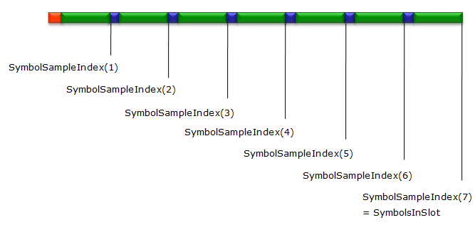
The slot structure the code has to follow. The CP lengths differ between the first symbol and the rest, so the symbol boundaries are not equally spaced.

The code below turns this structure into sample indices. SymbolSampleIndex is the cumulative sum of the CP and symbol lengths, so each entry marks the last sample of one OFDM symbol. The index of the last sample, minus Nfft - 1, gives the first sample after the CP.

% [160+2048;144+2048;144+2048;144+2048;144+2048;144+2048;144+2048]; represents the number of

% samples of Cyclic Prefix and OFDMA symbol data for each symbol with reference to 20 Mhz case show above

% (2048 IFFT bins, 30.72M sampling rate). For example, in case of 160 + 2048, 160 is the number of

% samples of the cyclic prefix of the first slot and 2048 is the number of samples of OFDMA symbol of the first

% slot.

% If System BW changes, the number of samples for data and cyclic prefix gets different. To figure out the

% number of samples for a specific BW from the 20 Mhz data, I create a variable SamplingScale

% SamplingScale is to scale the 20 Mhz case to the current BW that is being used.

 

SamplingScale = (double(tx_waveform_info.Nfft)/2048);

NoOfSampleList = SamplingScale * [160+2048;144+2048;144+2048;144+2048;144+2048;144+2048;144+2048];

 

% this is to convert the number in NoOfSampleList to represents the index number of each slot boundary.

 

SymbolSampleIndex = cumsum(NoOfSampleList);

 

% each elements of SymbolSampleIndex indicate the array index of the following positions.



 

% this is just to get the total number of data within a slot and store it in SymbolsInSlot

 

SymbolsInSlot = max(SymbolSampleIndex );

 

% You can specify the slot number for which you want to plot. since tx_waveform in this example carries 1 radio

% frame data, you can specifyvthe number 0~19 to this variable.

 

SlotNo = 2;

 

% tx_waveform contains all the samples within a radio frame in a single long one-dimensional array.

% In order to take out a chunk of a block of data corresponding to a specific OFDM symbol. We have to

% calculate the start and end of the sample index of the symbol. SymbolSampleIndexStart is the variable

% to store the index of the first sample in an OFDM symbol.

 

SymbolSampleIndexStart = 1;

 

% SymbolLength is the variable to store the number of samples contained in an OFDM symbol.

% Note that I used the function double() function to match the value type.

 

SymbolLength = double(tx_waveform_info.Nfft);

 

% Following for loop is to take out each OFDM symbol data from a specified slot and present it in plots.

% Each iteration will create two plots. The left plot would presents frequency domain plot for an OFDMA symbol

% the right plot would presents the time domain plot for an OFDMA symbol

 

for i = 1:7

 

    % plotIndex stores the array of the index within tx_waveform corresponding to all the samples for a specified

    % OFDM Symbol.

 

    plotIndex = (SymbolSampleIndex(i)+(1-SymbolLength:0)) + (SlotNo * SymbolsInSlot) ;

     

    % plotIndex for each 'i' value contains the indices for each symbol excluding Cyclic Prefix as shown below.



 

    % This is to take out all the samples for a specified (single) OFDM symbol and store the cut-out samples

    % to the variable symbolData

    

    symbolData=tx_waveform(plotIndex);

    symbolPlotData = 0.0 * (1:length(tx_waveform));

    symbolPlotData(1:length(symbolData)) = symbolData;

 

    % Following is to convert the time domain data to frequency domain data.

 

    freqData=fftshift(fft(symbolData));

    

    % Following is to plot of frequency domain data on the left side graph.

 

    subplot(7,5,5*(i-1)+1);

    plot(abs(freqData)); xlim([1 length(symbolData)]);%ylim([0 0.2]);

    set(gca,'xticklabel',[]); set(gca,'yticklabel',[]); set(gca,'xtick',[]); set(gca,'ytick',[]);

    

    % Following is to plot of time domain I-data on the left side graph.

 

    subplot(7,5,[5*(i-1)+2 5*(i-1)+3]);

    plot(real(tx_waveform(plotIndex))); xlim([1 length(plotIndex)]);ylim([-0.25 0.25]);

    set(gca,'xticklabel',[]); set(gca,'yticklabel',[]); set(gca,'xtick',[]); set(gca,'ytick',[]);

    ylabel(strcat('S',num2str(i-1),'-I'));

    

    % Following is to plot of time domain Q-data on the left side graph.

 

    subplot(7,5,[5*(i-1)+4 5*(i-1)+5]);

    plot(imag(tx_waveform(plotIndex))); xlim([1 length(plotIndex)]);ylim([-0.25 0.25]);

    set(gca,'xticklabel',[]); set(gca,'yticklabel',[]); set(gca,'xtick',[]); set(gca,'ytick',[]);

    ylabel(strcat('S',num2str(i-1),'-Q'));

 

    % Following is to move the value of SymbolSampleIndexStart to the start sample index of next OFDM Symbol

 

    SymbolSampleIndexStart = SymbolSampleIndex(i) + 1;

end;    

 

SymbolSampleIndex(7) equals SymbolsInSlot, the number of samples in one slot. Each loop step takes the last Nfft samples before SymbolSampleIndex(i), which is the symbol without its CP.

Each row of the plots below is one OFDM symbol. The left panel is the FFT magnitude of the symbol, with the zero frequency in the middle because of fftshift. The middle and right panels are the I and Q samples in the time domain.

Following example shows frequency and time domain I/Q data for the slot 0 (the first slot in 1st subframe) for System BW = 1.4 Mhz and PDSCH resource allocation of 4 RBs starting from RB 0. Examine each symbol plot (especially for frequency domain plot) and try to understand why you get such a plot.

 

enb.NDLRB = 6; START_RB = 0; N_RB = 4; SlotNo = 0;

 

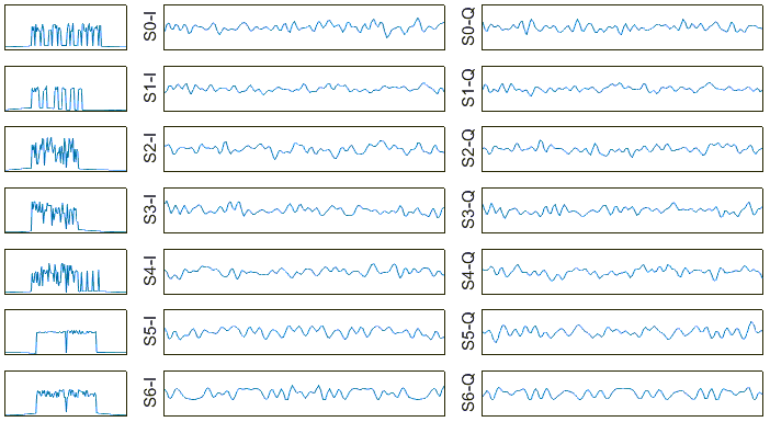
Slot 0 at 1.4 MHz. S0 and S1 are the control region, S2 to S4 carry the PDSCH on the lower 48 subcarriers, S5 is the SSS and S6 the PSS.

Following example shows frequency and time domain I/Q data for the slot 1 (the second slot in 1st subframe) for System BW = 1.4 Mhz and PDSCH resource allocation of 4 RBs starting from RB 0. Examine each symbol plot (especially for frequency domain plot) and try to understand why you get such a plot. Do you see any difference between this example and previous example ? What is the difference ? why you have such a difference ?

 

enb.NDLRB = 6; START_RB = 0; N_RB = 4; SlotNo = 1;

 

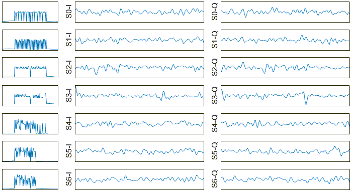
Slot 1 at 1.4 MHz. S0 to S3 are the PBCH across all 72 subcarriers, and S4 to S6 carry the PDSCH again.

Following example shows frequency and time domain I/Q data for the slot 2 (the first slot in 2nd subframe) for System BW = 1.4 Mhz and PDSCH resource allocation of 4 RBs starting from RB 0. Examine each symbol plot (especially for frequency domain plot) and try to understand why you get such a plot. Do you see any difference between this example and previous example ?

 

enb.NDLRB = 6; START_RB = 0; N_RB = 4; SlotNo = 2;

 

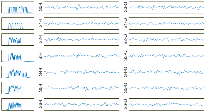
Slot 2 at 1.4 MHz, the first slot of subframe 1. There is no PSS, SSS or PBCH, so S2 to S6 all carry the PDSCH.

The spectra answer the questions in the text above. At 1.4 MHz, the control region takes two symbols even with CFI = 1, because 36.211 Table 6.7-1 uses CFI + 1 symbols when NDLRB is 10 or less. S0 and S1 therefore show the comb of the control channels across the whole carrier. The PDSCH on RB 0 to 3 fills only the lower 48 of the 72 subcarriers, so its spectrum stops about two thirds of the way across. S4 in slot 0 and slot 2 is wider, because it carries the CRS on all 6 RB.

Slot 0 and slot 1 differ because of the channels of subframe 0. Symbols 5 and 6 of slot 0 carry the SSS and the PSS, whose flat spectrum covers the central 62 subcarriers. Symbols 0 to 3 of slot 1 carry the PBCH, which covers all 72 subcarriers. Slot 2 belongs to subframe 1, which has none of these channels, so its symbols 2 to 6 show only the PDSCH.

Following example shows frequency and time domain I/Q data for the slot 0 (the first slot in 1st subframe) for System BW = 5 Mhz and PDSCH resource allocation of 4 RBs starting from RB 0. Examine each symbol plot (especially for frequency domain plot) and try to understand why you get such a plot.

 

enb.NDLRB = 25; START_RB = 0; N_RB = 4; SlotNo = 0;

 

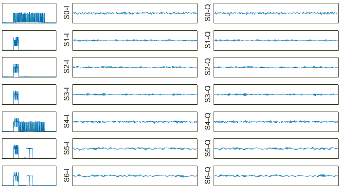
Slot 0 at 5 MHz. Only S0 is control. S1 to S3 carry the PDSCH at the lower edge, and S5 and S6 add the SSS and the PSS in the centre.

Following example shows frequency and time domain I/Q data for the slot 1 (the second slot in 1st subframe) for System BW = 5 Mhz and PDSCH resource allocation of 4 RBs starting from RB 0. Examine each symbol plot (especially for frequency domain plot) and try to understand why you get such a plot. Do you see any difference between this example and previous example ? What is the difference ? why you have such a difference ?

 

enb.NDLRB = 25; START_RB = 0; N_RB = 4; SlotNo = 1;

 

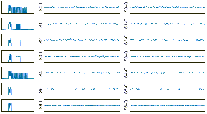
Slot 1 at 5 MHz. S0 to S3 add the PBCH in the central 72 subcarriers next to the PDSCH.

Following example shows frequency and time domain I/Q data for the slot 2 (the first slot in 2nd subframe) for System BW = 5 Mhz and PDSCH resource allocation of 4 RBs starting from RB 0. Examine each symbol plot (especially for frequency domain plot) and try to understand why you get such a plot. Do you see any difference between this example and previous example ?

 

enb.NDLRB = 25; START_RB = 0; N_RB = 4; SlotNo = 2;

 

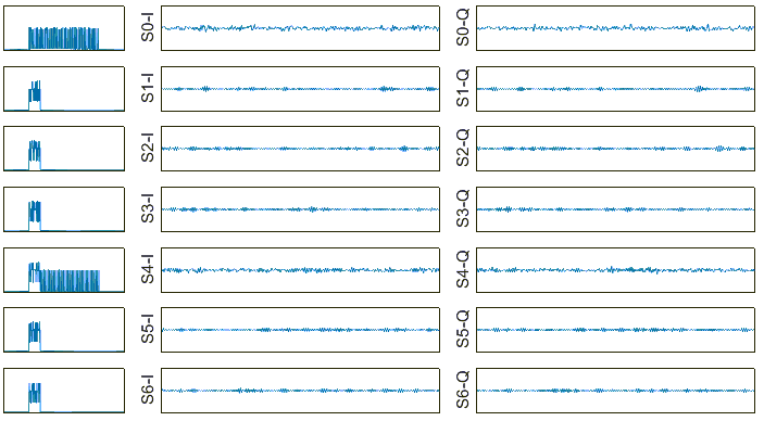
Slot 2 at 5 MHz. The PDSCH alone at the lower edge in S1 to S6, with the CRS across the band in S4.

At 5 MHz the carrier has 25 RB, so two things change. First, the control region is one symbol, because CFI = 1 now means 1 symbol. S1 of slot 0 therefore already carries the PDSCH. Second, the 4 PDSCH RBs are now a small part of the carrier, and the PSS, SSS and PBCH take only the central 6 RB. The spectra show them as separate blocks, the PDSCH at the lower edge and the synchronization signals or the PBCH in the centre.

The time domain panels change too. The amplitude of an OFDM symbol grows with the number of subcarriers it carries. At 5 MHz, the symbols with only 48 active subcarriers have a much smaller swing than S0 and S4, which carry the control channels or the CRS across all 300 subcarriers.

• SymbolSampleIndex marks the end of each symbol : the last Nfft samples are the symbol without its CP.
• 1.4 MHz: 2 control symbols with CFI 1 : 36.211 Table 6.7-1 for NDLRB of 10 or less.
• Slot 0 and slot 1 carry SSS, PSS and PBCH : slot 2 carries only control and PDSCH.
• 5 MHz: 1 control symbol : the PDSCH and the central channels appear as separate blocks.

Plotting Resource Grid and Time Domain for whole Radio Frame

One slot shows 7 symbols. This section repeats the extraction for all 20 slots of the frame, so the FFT of every symbol can be stacked into a picture of the whole resource grid, recovered from the waveform.

This is a extension of the previous section. In previous section, I plotted the time domain and frequency domain for each OFDM symbol separately for one slot. In this section, I will repeat the previous process for all slots (20 slots) within a radio frame and plot them all together.

% [160+2048;144+2048;144+2048;144+2048;144+2048;144+2048;144+2048]; represents the number of

% samples of Cyclic Prefix and OFDMA symbol data for each symbol with reference to 20 Mhz case

% (2048 IFFT bins, 30.72M sampling rate). For example, in case of 160 + 2048, 160 is the number of

% samples of the cyclic prefix of the first slot and 2048 is the number of samples of OFDMA symbol of the first

% slot.

% SamplingScale is to scale the 20 Mhz case to the current BW that is being used.

 

SamplingScale = (double(tx_waveform_info.Nfft)/2048);

NoOfSampleList = SamplingScale * [160+2048;144+2048;144+2048;144+2048;144+2048;144+2048;144+2048];

 

% this is to convert the number in NoOfSampleList to represents the index number of each slot boundary.

 

SymbolSampleIndex = cumsum(NoOfSampleList);

 

% this is just to get the total number of data within a slot and store it in SymbolsInSlot

 

SymbolsInSlot = max(SymbolSampleIndex );

 

% Create three variables (empty arrays) to store the frequency domain, I/Q data

 

SpectrumList = [];

TimeDomainListI = [];

TimeDomainListQ = [];

 

% You can specify the slot number for which you want to plot.

% Since tx_waveform in this example carries 1 radio frame data, you can specify the number 0~19 to this

% variable.

 

for SlotNo = 0:19

 

% tx_waveform contains all the samples within a radio frame in a single long one-dimensional array.

% In order to take out a chunk of a block of data corresponding to a specific OFDM symbol. We have to

% calculate the start and end of the sample index of the symbol. SymbolSampleIndexStart is the variable

% to store the index of the first sample in an OFDM symbol.

 

SymbolSampleIndexStart = 1;

 

% SymbolLength is the variable to store the number of samples contained in an OFDM symbol.

% Note that I used the function double() function to match the value type.

 

SymbolLength = double(tx_waveform_info.Nfft);

 

% Following for loop is to take out each OFDM symbol data from a slot and do following procedure

%       i) convert it to frequency domain and add the data to SpectrumList[]

%       ii) take out I component and add the data to TimeDomainListI[]

%       iii) take out I component and add the data to TimeDomainListQ[]

 

for i = 1:7

 

    % plotIndex stores the array of the index within tx_waveform corresponding to all the samples

    % for a specified OFDM Symbol.

 

    plotIndex = (SymbolSampleIndex(i)+(1-SymbolLength:0)) + (SlotNo * SymbolsInSlot) ;

    

    % This is to take out all the samples for a specified (single) OFDM symbol and store the cut-out samples

    % to the variable symbolData

 

    symbolData=tx_waveform(plotIndex);

    symbolPlotData = 0.0 * (1:length(tx_waveform));

    symbolPlotData(1:length(symbolData)) = symbolData;

 

    % Following is to convert the time domain data to frequency domain data.

 

    freqData=fftshift(fft(symbolData));

    

    % add (store) the frequency domain data to SpectrumList[]

 

    SpectrumList = [SpectrumList ; abs(freqData)'];

 

    % add (store) the time domain I data to TimeDomainListI[]

 

    TimeDomainListI = [TimeDomainListI;real(tx_waveform(plotIndex))'];

    

    % add (store) the time domain Q data  to TimeDomainListQ[]

 

     TimeDomainListQ = [TimeDomainListQ;imag(tx_waveform(plotIndex))'];

 

    % Following is to move the value of SymbolSampleIndexStart to the start sample index of next OFDM

    % Symbol

 

    SymbolSampleIndexStart = SymbolSampleIndex(i) + 1;

end;    

 

end;

 

% Following is to plot the resource grid for the whole radio frame.

 

subplot(2,2,[1 2]);

surface(SpectrumList','FaceColor','flat','EdgeColor','none'); zlim([0 3.5]); xlim([1 140]); ylim([1 SymbolLength]); view([0,90]);

 

% Following is to plot time domain I data for the whole radio frame.

 

subplot(2,2,3);

waterfall(TimeDomainListI'); zlim([-0.25 0.25]); ylim([1 140]);

ylim([1 SymbolLength]); xlabel('Symbol index'); ylabel('Sample index');  view([-40,45]);

 

% Following is to plot time domain Q data for the whole radio frame.

 

subplot(2,2,4);

waterfall(TimeDomainListQ'); zlim([-0.25 0.25]); ylim([1 140]);

ylim([1 SymbolLength]); xlabel('Symbol index'); ylabel('Sample index');  view([-40,45]);

 

Following is the example for plotting frequency and I/Q data plot for the whole radion frame for BW = 1.4 MHz and and PDSCH resource allocation of 4 RBs starting from RB 0

 

enb.NDLRB = 6; START_RB = 0; N_RB = 4;

 

The whole frame at 1.4 MHz. The upper plot is the FFT magnitude of all 140 symbols over the 128 FFT bins. The lower plots are the in-phase and quadrature samples of each symbol.

Following is the example for plotting frequency and I/Q data plot for the whole radion frame for BW = 5 MHz and and PDSCH resource allocation of 4 RBs starting from RB 0

 

enb.NDLRB = 25; START_RB = 0; N_RB = 4;

 

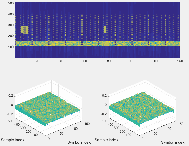
The whole frame at 5 MHz, over 512 FFT bins. The PDSCH is the dense band at the lower edge of the carrier, and the PSS, SSS and PBCH are the blocks in the centre.

The upper plots are the resource grid of the first section, recovered from the time domain samples. The occupied band is 72 subcarriers of the 128 bins at 1.4 MHz, and 300 subcarriers of the 512 bins at 5 MHz. The rest of the bins are the zero padding that lteOFDMModulate adds. A thin dark line runs through the middle of the band at 1.4 MHz. That is the DC subcarrier, which LTE leaves empty in the downlink.

The blocks near the start of the frame are subframe 0: the SSS and PSS in symbols 5 and 6, and the PBCH in symbols 7 to 10. A second, narrower block appears around symbol 76, which is symbols 5 and 6 of subframe 5, where the PSS and SSS repeat. The PBCH does not repeat there, because it is sent only in subframe 0. The narrow columns that repeat every 14 symbols are the control region at the start of each subframe.

• The FFT of each symbol rebuilds the resource grid : 140 symbols per frame.
• Zero padding outside the occupied band : the empty bins above and below the carrier.
• PSS and SSS in subframes 0 and 5 : PBCH only in subframe 0.

Plotting Frequency Spectrum

The last view is the one a spectrum analyzer shows. It averages the power over the whole frame, so it shows how the power is spread across the carrier rather than which channel sits where.

In this last section, I will show you how to display the radio frame time domain data stored in tx_waveform in spectrum analyzer. Method is very simple. Just pass the data into dsp.SpectrumAnalyzer(), but I added a short procedure to figure out the frequency span from enb parameter.

% following is to figure out RF bandwidth in Hz from enb parameter (enb.NDLRB)

if enb.NDLRB == 6

   span = 1.4e6;

end;

 

if enb.NDLRB == 15

   span = 3.0e6;

end;

 

if enb.NDLRB == 25

   span = 5.0e6;

end;

 

if enb.NDLRB == 50

   span = 10.0e6;

end;

 

if enb.NDLRB == 75

   span = 15.0e6;

end;

 

if enb.NDLRB == 100

   span = 20.0e6;

end;

 

% Following is to create a spectrum analyzer instances with proper configuration for displaying the tx_waveform

% Green part is something you have to pay attention and may want to change as you want.

 

hSpecAnalTx = dsp.SpectrumAnalyzer('SampleRate', tx_waveform_info.SamplingRate, ...

    'SpectrumType', 'Power density', 'PowerUnits', 'dBm', ...

    'RBWSource', 'Property','RBW', 1.5e3, ...

    'FrequencySpan', 'Span and center frequency', ...

    'Span', span, 'CenterFrequency', 0, ...

    'Window', 'Hamming', 'SpectralAverages', 20, ...

    'YLimits', [-100 -40], 'YLabel', 'PSD', ...

    'Title', 'LTE Downlink Transmission Spectrum', ...

    'ShowLegend', false);

 

% Following is to pass the data into spectrum analyzer that was created above.

 

step(hSpecAnalTx, tx_waveform);

 

enb.NDLRB = 6; enb.CellRefP = 1; enb.NCellID = 0; START_RB = 0; N_RB = 4;
tx_waveform_info =     SamplingRate: 1920000             Nfft: 128        Windowing: 4

 

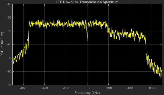
The spectrum of the 1.4 MHz frame. The PSD is about 9 dB higher from -540 kHz to +180 kHz, where the PDSCH on RB 0 to 3 is. The notch at 0 kHz is the empty DC subcarrier.

The if chain maps NDLRB to the channel bandwidth of 36.101 Table 5.6-1, for example 6 RB to 1.4 MHz and 25 RB to 5 MHz. The 6 RB carry 72 subcarriers of 15 kHz, which is 1.08 MHz, so the signal occupies about -540 kHz to +540 kHz inside the 1.4 MHz span. The rest of the channel bandwidth is guard band.

RB 0 is at the lowest frequency, so the 4 PDSCH RBs cover -540 kHz to +180 kHz. That part carries data in every symbol outside the control region, and its PSD sits near -53 dBm/Hz. RB 4 and RB 5 carry only the CRS, the control channels and, in subframes 0 and 5, the synchronization signals and the PBCH. Their average PSD is therefore about 9 dB lower.

The analyzer settings shape what the plot can resolve. RBW = 1.5 kHz is a tenth of the 15 kHz subcarrier spacing, so the DC notch, one subcarrier wide, stays visible. SpectralAverages = 20 averages over many symbols, which smooths the PSD of the random PDSCH data into a flat level. The sample rate comes from tx_waveform_info.SamplingRate, 1.92 MHz here, so the analyzer can show at most 1.92 MHz around the carrier, and the 1.4 MHz span fits inside it.

Outside the occupied band, the PSD falls by 15 to 20 dB at the band edge and then keeps sloping down. The waveform has no transmit filter. Only the raised cosine windowing of lteOFDMModulate, 4 samples here as tx_waveform_info.Windowing shows, softens the symbol edges. A real transmitter adds filtering to meet the emission masks of 36.101, so this plot shows the OFDM signal itself rather than a compliant RF output.

• Span from the channel bandwidth : 36.101 Table 5.6-1 maps NDLRB to MHz.
• 1.08 MHz occupied at 1.4 MHz : 72 subcarriers of 15 kHz.
• The PDSCH RBs stand out : about 9 dB above RB 4 and RB 5.
• No transmit filter : only 4 samples of windowing shape the band edges.

Disclaimer !

This page is only to show you the overall logics and visualization for various LTE physical layer channels. I haven't investigated much about verifying about the accuracy.

If you think the code is not so efficient, it is 100% my fault. I haven't made any effort for effiecient code. I just tried to create code as simple as possible for the readers. As you know, easy-to-read code is not always efficient for a specific chipset.

If you find any mistake in terms of accuracy, it is also very highly likely be my fault. Not the problem of Matlab tool box itself.

Any comment and corrections if you find any mistake will be welcome and appreciated.

Reference

[1] 3GPP TS 36.211 v19.3.0 - clause 6.12, OFDM baseband signal generation, Table 6.12-1, and Table 6.7-1, Number of OFDM symbols used for PDCCH

[2] 3GPP TS 36.101 v20.0.0 - Table 5.6-1, Transmission bandwidth configuration N_RB in E-UTRA channel bandwidths