In this page, I will show you how OFDM demodulation works by using 'semi-real data'. By semi-real, I mean that the data that I used here is not from live eNB but generated by a real hardware (Vector signal generator) and captured by Vector Signal Analyzer with special Sync signal. So you don't have to implement an algorithm for synchronization and a lot of compensation which is a too much for an example. If you are interested in working as beginner level of LTE DSP, this can be helpful or motivation as well.
The demodulation itself is short. The receiver drops the cyclic prefix, takes a 512 point FFT of each OFDM symbol, and reads the resource elements off the FFT bins. The page shows the result first, then the signal configuration, and then the Matlab code that produced the result.
Followings are the topics to be covered in this page.
Result
Can a plain FFT recover the LTE resource grid, if the timing is already known? The figure below answers that for the seven OFDM symbols of slot 0 in subframe 0. Each row is one symbol, and each column is one stage of the processing.
Following is the result of the Matlab source code listed here. (A) shows the frequency domain result for each symbols within the first slot of subframe 0. (B) is the I/Q plot (real and imaginary) representation of column (A). You would notice some degree of rotation (phase shift). (C) is the result after phase compensation of column (B).
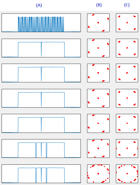
Rows are OFDM symbols 0 to 6 of slot 0. Column (A) is the FFT magnitude, column (B) the raw constellation, and column (C) the constellation after the fixed phase rotation.
Symbol 0 : a comb-like spectrum, because only part of the resource elements carry energy in the control region.Symbols 1 to 4 : a flat block of 300 subcarriers with a notch at DC, and four clean QPSK clusters.Symbol 5 : narrow gaps appear around the centre of the spectrum, and extra points appear in the constellation.Symbol 6 : the same centre gaps, and a ring of points in the constellation.The point at the origin : the DC subcarrier and the unused FFT bins outside the 300 subcarriers.
The last two rows differ from the others because of the synchronization signals. For frame structure type 1, 36.211 v19.3.0 clause 6.11 maps the PSS to the last OFDM symbol of slots 0 and 10, and the SSS to the symbol before it. Both use the 62 subcarriers around DC, with 5 reserved subcarriers on each side. Those reserved subcarriers are the narrow gaps in column (A) for symbols 5 and 6.
The constellations show the same signals. The SSS is built from binary sequences, so its values are real. After compensation, they form two extra clusters on the real axis in column (C) for symbol 5. The PSS is a Zadoff-Chu sequence, which has a constant amplitude and a changing phase. Its values therefore spread around a circle in symbol 6, while the data around it stays in the four QPSK clusters.
One fixed PhaseOffset corrects all seven symbols. So the phase does not drift over the 0.5 ms slot, and the residual frequency offset between the signal generator and the analyzer is small. The rotation in column (B) is only a common phase, which a real receiver would remove with the cell-specific reference signals.
PSS in symbol 6, SSS in symbol 5 : the last two symbols of slot 0 for FDD.SSS values are real : two clusters on the real axis after compensation.PSS values have constant amplitude : a ring in the constellation.One phase value fits every symbol : no visible frequency drift over the slot.
LTE Configuration of the Data
The FFT output makes sense only against the configuration of the signal. The bandwidth sets the number of occupied subcarriers, and the CFI sets which symbols carry the control region. The signal generator used the following settings.
The data that I used in this example is from following LTE Configuration.
- System BandWidth = 5 Mhz
- Number of RB = 25
- Physical Cell ID = 0
- CFI = 1
- Sampling Rate = 7.68 Mhz
A 5 MHz LTE carrier has 25 RB, which is 300 subcarriers of 15 kHz. The file name of the data, LTE_DL_5M_25RB_S_7_68_SG_Trig.bin, carries the same 25 RB. At 7.68 Msps, the FFT has 512 bins, so 212 bins outside the carrier and the DC bin carry no data. After fftshift, the carrier occupies bins 107 to 407, which is the flat block in column (A).
CFI = 1 means the control region is one OFDM symbol long. So symbol 0 carries the whole control region: the reference signals, PCFICH, PHICH and PDCCH. Many resource elements of this symbol carry no energy in this signal, and that gives the symbol 0 spectrum its comb shape. Physical Cell ID = 0 selects the PSS and SSS sequences and the position of the reference signals.
25 RB : 300 subcarriers, bins 107 to 407 of 512.7.68 Msps : a quarter of the 30.72 Msps reference rate.CFI = 1 : symbol 0 is the only control symbol.Physical Cell ID = 0 : sets the PSS, the SSS and the reference signal pattern.
Matlab Code
The code has to answer two questions before any FFT is taken: where each OFDM symbol starts, and how many samples its cyclic prefix has. The first answer is a given number here. The second comes from the LTE numerology, scaled from 20 MHz down to 5 MHz.
Following is the Matlab source code that produced the figure shown above. The code is designed intentionally long. I might have make it very short if I used for-loop, but it would look harder to understand. So I try to write every procedure step by step. Hopefully, this would be easier for you to follow even though it looks a little too lengthy.
clear all;
% you can download the data file in this example from here.
% this is for reading the baseband IQ data of OFDM symbol in time domain.
% detailed explantion for this three line and file format in this example is described in
% Matlab : Read Number in Binary file page.
fid = fopen('LTE_DL_5M_25RB_S_7_68_SG_Trig.bin','r');
[data,count] = fread(fid, 'single');
fclose(fid);
% This variable represents the first sample in the first OFDM symbol.
% How do I know this ? This is just a magic number I could figure out from the vector signal
% analyzer. Just think this is just a given number. If you seriously want to work in this
% area, try to implement the algorithm to find this number on your own.
Offset = 280228 + 2 ;
% Nfft represents the FFT size for the specified system bandwidth. 512 is the FFT size for
% 5 Mhz System Bandwidth.
Nfft = 512;
% SamplingScale is to figure out the number of samples in CP and OFDM Symbol for each specific system
% Bandwidth from the 20 Mhz Bandwidth. Physical Layer Parameters - FDD, Downlink will help you understand
% the meaning of each numbers here.
SamplingScale = (double(Nfft)/2048);
CP_LengthList = SamplingScale * [160;144;144;144;144;144;144];
Symbol_LengthList = SamplingScale * [2048;2048;2048;2048;2048;2048;2048];
% This is to compensate the phase rotation shown in track (B) of the result.
% How do I figure out this number. I just got it by eye balling and a couple of try and error.
% If you seriously want to work in this area, try to implement the algorithm to find this
% number on your own.
PhaseOffset = exp(-j*pi/2.5)
%%%%%%%%%%%%%%%%%%%%%%%%%%%%%% Demodulation of symbol 0 %%%%%%%%%%%%%%%%%%%%%%%%%%%%%%%%%%%
% This is to demoulate the symbol 0 within the slot 0 of Subframe 0.
% ChuckStart here indicates the index(position) of the first sample within the binary file.
% You would notice that I skip the first CP length. This is the same effect of removing the
% first CP as described in CP removal described in RE Map to/from Antenna page.
ChunkStart = Offset ...
+ CP_LengthList(1);
% This variable indicates the number of samples within the first OFDM symbol excluding the CP
ChunkLength = Symbol_LengthList(1);
% This is to read I/Q data pair.
DataChunk = data(2*ChunkStart-1:2*(ChunkStart+ChunkLength));
% This is to separate I and Q into a separate array (vector)
DataChunkI = DataChunk(1:2:length(DataChunk));
DataChunkQ = DataChunk(2:2:length(DataChunk));
% This is to combine I array and Q array into a complex number array.
DataChunkComplex = DataChunkI + j*DataChunkQ;
% This is to convert the time domain OFDM Symbol into Frequency Domain and Normalize it.
DataChunkFFT = fftshift(fft(DataChunkComplex,Nfft));
DataChunkFFT = DataChunkFFT/max(abs(DataChunkFFT));
DataChunkFftMag = abs(DataChunkFFT);
% This is to plot the FFT result in magnitude.
% The result of this block is shown in track (A) of the figure at the beginning of the page
subplot(7,5,[1 3]);
plot(DataChunkFftMag);xlim([1, length(DataChunkFftMag)]); ylim([0 1.2]);
set(gca,'xticklabel',[]);set(gca,'yticklabel',[]);
set(gca,'xtick',[]);set(gca,'ytick',[]);
% This is to plot the FFT result in complex domain (I and Q axis)
% The result of this block is shown in track (B) of the figure at the beginning of the page
subplot(7,5,4);
plot(real(DataChunkFFT),imag(DataChunkFFT),'ro','MarkerFaceColor',[1 0 0],'MarkerSize',2);
xlim([-1 1]);ylim([-1 1]);
set(gca,'xticklabel',[]);set(gca,'yticklabel',[]);
set(gca,'xtick',[]);set(gca,'ytick',[]);
% This is to plot the FFT result rotated by the angle specified by the variable PhaseOffset
% The result of this block is shown in track (C) of the figure at the beginning of the page
subplot(7,5,5);
DataChunkFFT_Comp = DataChunkFFT .* PhaseOffset;
plot(real(DataChunkFFT_Comp),imag(DataChunkFFT_Comp),'ro','MarkerFaceColor',[1 0 0],'MarkerSize',2);
xlim([-1 1]);ylim([-1 1]);
set(gca,'xticklabel',[]);set(gca,'yticklabel',[]);
set(gca,'xtick',[]);set(gca,'ytick',[]);
%%%%%%%%%%%%%%%%%%%%%%%%%%%%%% Demodulation of symbol 1 %%%%%%%%%%%%%%%%%%%%%%%%%%%%%%%%%%%
% This is to demodulate the symbol 1 within the slot 0 of Subframe 0. Everything is same
% as in the symbol 0 analysis except the 'ChunkStart. So I would not explain any further.
ChunkStart = Offset ...
+ CP_LengthList(1) + Symbol_LengthList(1) ...
+ CP_LengthList(2) ;
ChunkLength = Symbol_LengthList(2);
DataChunk = data(2*ChunkStart-1:2*(ChunkStart+ChunkLength));
DataChunkI = DataChunk(1:2:length(DataChunk));
DataChunkQ = DataChunk(2:2:length(DataChunk));
DataChunkComplex = DataChunkI + j*DataChunkQ;
DataChunkFFT = fftshift(fft(DataChunkComplex,Nfft));
DataChunkFFT = DataChunkFFT/max(abs(DataChunkFFT));
DataChunkFftMag = abs(DataChunkFFT);
subplot(7,5,[6 8]);
plot(DataChunkFftMag);xlim([1, length(DataChunkFftMag)]); ylim([0 1.2]);
set(gca,'xticklabel',[]);set(gca,'yticklabel',[]);
set(gca,'xtick',[]);set(gca,'ytick',[]);
subplot(7,5,9);
plot(real(DataChunkFFT),imag(DataChunkFFT),'ro','MarkerFaceColor',[1 0 0],'MarkerSize',2);
xlim([-1 1]);ylim([-1 1]);
set(gca,'xticklabel',[]);set(gca,'yticklabel',[]);
set(gca,'xtick',[]);set(gca,'ytick',[]);
subplot(7,5,10);
DataChunkFFT_Comp = DataChunkFFT .* PhaseOffset;
plot(real(DataChunkFFT_Comp),imag(DataChunkFFT_Comp),'ro','MarkerFaceColor',[1 0 0],'MarkerSize',2);
xlim([-1 1]);ylim([-1 1]);
set(gca,'xticklabel',[]);set(gca,'yticklabel',[]);
set(gca,'xtick',[]);set(gca,'ytick',[]);
%%%%%%%%%%%%%%%%%%%%%%%%%%%%%% Demodulation of symbol 2 %%%%%%%%%%%%%%%%%%%%%%%%%%%%%%%%%%%
% This is to demodulate the symbol 2 within the slot 0 of Subframe 0. Everything is same
% as in the symbol 0 analysis except the 'ChunkStart. So I would not explain any further.
ChunkStart = Offset ...
+ CP_LengthList(1) + Symbol_LengthList(1) ...
+ CP_LengthList(2) + Symbol_LengthList(2) ...
+ CP_LengthList(3);
ChunkLength = Symbol_LengthList(3);
DataChunk = data(2*ChunkStart-1:2*(ChunkStart+ChunkLength));
DataChunkI = DataChunk(1:2:length(DataChunk));
DataChunkQ = DataChunk(2:2:length(DataChunk));
DataChunkComplex = DataChunkI + j*DataChunkQ;
DataChunkFFT = fftshift(fft(DataChunkComplex,Nfft));
DataChunkFFT = DataChunkFFT/max(abs(DataChunkFFT));
DataChunkFftdB = abs(DataChunkFFT);
subplot(7,5,[11 13]);
plot(DataChunkFftdB);xlim([1, length(DataChunkFftdB)]); ylim([0 1.2]);
set(gca,'xticklabel',[]);set(gca,'yticklabel',[]);
set(gca,'xtick',[]);set(gca,'ytick',[]);
subplot(7,5,14);
plot(real(DataChunkFFT),imag(DataChunkFFT),'ro','MarkerFaceColor',[1 0 0],'MarkerSize',2);
xlim([-1 1]);ylim([-1 1]);
set(gca,'xticklabel',[]);set(gca,'yticklabel',[]);
set(gca,'xtick',[]);set(gca,'ytick',[]);
subplot(7,5,15);
DataChunkFFT_Comp = DataChunkFFT .* PhaseOffset;
plot(real(DataChunkFFT_Comp),imag(DataChunkFFT_Comp),'ro','MarkerFaceColor',[1 0 0],'MarkerSize',2);
xlim([-1 1]);ylim([-1 1]);
set(gca,'xticklabel',[]);set(gca,'yticklabel',[]);
set(gca,'xtick',[]);set(gca,'ytick',[]);
%%%%%%%%%%%%%%%%%%%%%%%%%%%%%% Demodulation of symbol 3 %%%%%%%%%%%%%%%%%%%%%%%%%%%%%%%%%%%
% This is to demodulate the symbol 3 within the slot 0 of Subframe 0. Everything is same
% as in the symbol 0 analysis except the 'ChunkStart. So I would not explain any further.
ChunkStart = Offset ...
+ CP_LengthList(1) + Symbol_LengthList(1) ...
+ CP_LengthList(2) + Symbol_LengthList(2) ...
+ CP_LengthList(3) + Symbol_LengthList(3) ...
+ CP_LengthList(4);
ChunkLength = Symbol_LengthList(4);
DataChunk = data(2*ChunkStart-1:2*(ChunkStart+ChunkLength));
DataChunkI = DataChunk(1:2:length(DataChunk));
DataChunkQ = DataChunk(2:2:length(DataChunk));
DataChunkComplex = DataChunkI + j*DataChunkQ;
DataChunkFFT = fftshift(fft(DataChunkComplex,Nfft));
DataChunkFFT = DataChunkFFT/max(abs(DataChunkFFT));
DataChunkFftdB = abs(DataChunkFFT);
subplot(7,5,[16 18]);
plot(DataChunkFftdB);xlim([1, length(DataChunkFftdB)]); ylim([0 1.2]);
set(gca,'xticklabel',[]);set(gca,'yticklabel',[]);
set(gca,'xtick',[]);set(gca,'ytick',[]);
subplot(7,5,19);
plot(real(DataChunkFFT),imag(DataChunkFFT),'ro','MarkerFaceColor',[1 0 0],'MarkerSize',2);
xlim([-1 1]);ylim([-1 1]);
set(gca,'xticklabel',[]);set(gca,'yticklabel',[]);
set(gca,'xtick',[]);set(gca,'ytick',[]);
subplot(7,5,20);
DataChunkFFT_Comp = DataChunkFFT .* PhaseOffset;
plot(real(DataChunkFFT_Comp),imag(DataChunkFFT_Comp),'ro','MarkerFaceColor',[1 0 0],'MarkerSize',2);
xlim([-1 1]);ylim([-1 1]);
set(gca,'xticklabel',[]);set(gca,'yticklabel',[]);
set(gca,'xtick',[]);set(gca,'ytick',[]);
%%%%%%%%%%%%%%%%%%%%%%%%%%%%%% Demodulation of symbol 4 %%%%%%%%%%%%%%%%%%%%%%%%%%%%%%%%%%%
% This is to demodulate the symbol 4 within the slot 0 of Subframe 0. Everything is same
% as in the symbol 0 analysis except the 'ChunkStart. So I would not explain any further.
ChunkStart = Offset ...
+ CP_LengthList(1) + Symbol_LengthList(1) ...
+ CP_LengthList(2) + Symbol_LengthList(2) ...
+ CP_LengthList(3) + Symbol_LengthList(3) ...
+ CP_LengthList(4) + Symbol_LengthList(4) ...
+ CP_LengthList(5);
ChunkLength = Symbol_LengthList(5);
DataChunk = data(2*ChunkStart-1:2*(ChunkStart+ChunkLength));
DataChunkI = DataChunk(1:2:length(DataChunk));
DataChunkQ = DataChunk(2:2:length(DataChunk));
DataChunkComplex = DataChunkI + j*DataChunkQ;
DataChunkFFT = fftshift(fft(DataChunkComplex,Nfft));
DataChunkFFT = DataChunkFFT/max(abs(DataChunkFFT));
DataChunkFftdB = abs(DataChunkFFT);
subplot(7,5,[21 23]);
plot(DataChunkFftdB);xlim([1, length(DataChunkFftdB)]); ylim([0 1.2]);
set(gca,'xticklabel',[]);set(gca,'yticklabel',[]);
set(gca,'xtick',[]);set(gca,'ytick',[]);
subplot(7,5,24);
plot(real(DataChunkFFT),imag(DataChunkFFT),'ro','MarkerFaceColor',[1 0 0],'MarkerSize',2);
xlim([-1 1]);ylim([-1 1]);
set(gca,'xticklabel',[]);set(gca,'yticklabel',[]);
set(gca,'xtick',[]);set(gca,'ytick',[]);
subplot(7,5,25);
DataChunkFFT_Comp = DataChunkFFT .* PhaseOffset;
plot(real(DataChunkFFT_Comp),imag(DataChunkFFT_Comp),'ro','MarkerFaceColor',[1 0 0],'MarkerSize',2);
xlim([-1 1]);ylim([-1 1]);
set(gca,'xticklabel',[]);set(gca,'yticklabel',[]);
set(gca,'xtick',[]);set(gca,'ytick',[]);
%%%%%%%%%%%%%%%%%%%%%%%%%%%%%% Demodulation of symbol 5 %%%%%%%%%%%%%%%%%%%%%%%%%%%%%%%%%%%
% This is to demodulate the symbol 5 within the slot 0 of Subframe 0. Everything is same
% as in the symbol 0 analysis except the 'ChunkStart. So I would not explain any further.
ChunkStart = Offset ...
+ CP_LengthList(1) + Symbol_LengthList(1) ...
+ CP_LengthList(2) + Symbol_LengthList(2) ...
+ CP_LengthList(3) + Symbol_LengthList(3) ...
+ CP_LengthList(4) + Symbol_LengthList(4) ...
+ CP_LengthList(5) + Symbol_LengthList(5) ...
+ CP_LengthList(6);
ChunkLength = Symbol_LengthList(6);
DataChunk = data(2*ChunkStart-1:2*(ChunkStart+ChunkLength));
DataChunkI = DataChunk(1:2:length(DataChunk));
DataChunkQ = DataChunk(2:2:length(DataChunk));
DataChunkComplex = DataChunkI + j*DataChunkQ;
DataChunkFFT = fftshift(fft(DataChunkComplex,Nfft));
DataChunkFFT = DataChunkFFT/max(abs(DataChunkFFT));
DataChunkFftdB = abs(DataChunkFFT);
subplot(7,5,[26 28]);
plot(DataChunkFftdB);xlim([1, length(DataChunkFftdB)]); ylim([0 1.2]);
set(gca,'xticklabel',[]);set(gca,'yticklabel',[]);
set(gca,'xtick',[]);set(gca,'ytick',[]);
subplot(7,5,29);
plot(real(DataChunkFFT),imag(DataChunkFFT),'ro','MarkerFaceColor',[1 0 0],'MarkerSize',2);
xlim([-1 1]);ylim([-1 1]);
set(gca,'xticklabel',[]);set(gca,'yticklabel',[]);
set(gca,'xtick',[]);set(gca,'ytick',[]);
subplot(7,5,30);
DataChunkFFT_Comp = DataChunkFFT .* PhaseOffset;
plot(real(DataChunkFFT_Comp),imag(DataChunkFFT_Comp),'ro','MarkerFaceColor',[1 0 0],'MarkerSize',2);
xlim([-1 1]);ylim([-1 1]);
set(gca,'xticklabel',[]);set(gca,'yticklabel',[]);
set(gca,'xtick',[]);set(gca,'ytick',[]);
%%%%%%%%%%%%%%%%%%%%%%%%%%%%%% Demodulation of symbol 6 %%%%%%%%%%%%%%%%%%%%%%%%%%%%%%%%%%%
% This is to demodulate the symbol 6 within the slot 0 of Subframe 0. Everything is same
% as in the symbol 0 analysis except the 'ChunkStart. So I would not explain any further.
ChunkStart = Offset ...
+ CP_LengthList(1) + Symbol_LengthList(1) ...
+ CP_LengthList(2) + Symbol_LengthList(2) ...
+ CP_LengthList(3) + Symbol_LengthList(3) ...
+ CP_LengthList(4) + Symbol_LengthList(4) ...
+ CP_LengthList(5) + Symbol_LengthList(5) ...
+ CP_LengthList(6) + Symbol_LengthList(6) ...
+ CP_LengthList(7);
ChunkLength = Symbol_LengthList(7);
DataChunk = data(2*ChunkStart-1:2*(ChunkStart+ChunkLength));
DataChunkI = DataChunk(1:2:length(DataChunk));
DataChunkQ = DataChunk(2:2:length(DataChunk));
DataChunkComplex = DataChunkI + j*DataChunkQ;
DataChunkFFT = fftshift(fft(DataChunkComplex,Nfft));
DataChunkFFT = DataChunkFFT/max(abs(DataChunkFFT));
DataChunkFftdB = abs(DataChunkFFT);
subplot(7,5,[31 33]);
plot(DataChunkFftdB);xlim([1, length(DataChunkFftdB)]); ylim([0 1.2]);
set(gca,'xticklabel',[]);set(gca,'yticklabel',[]);
set(gca,'xtick',[]);set(gca,'ytick',[]);
subplot(7,5,34);
plot(real(DataChunkFFT),imag(DataChunkFFT),'ro','MarkerFaceColor',[1 0 0],'MarkerSize',2);
xlim([-1 1]);ylim([-1 1]);
set(gca,'xticklabel',[]);set(gca,'yticklabel',[]);
set(gca,'xtick',[]);set(gca,'ytick',[]);
subplot(7,5,35);
DataChunkFFT_Comp = DataChunkFFT .* PhaseOffset;
plot(real(DataChunkFFT_Comp),imag(DataChunkFFT_Comp),'ro','MarkerFaceColor',[1 0 0],'MarkerSize',2);
xlim([-1 1]);ylim([-1 1]);
set(gca,'xticklabel',[]);set(gca,'yticklabel',[]);
set(gca,'xtick',[]);set(gca,'ytick',[]);
The scaling works as follows. SamplingScale is 512/2048 = 0.25. So the cyclic prefix is 160 × 0.25 = 40 samples for the first symbol of the slot, and 144 × 0.25 = 36 samples for the others. Each symbol has 512 samples after the cyclic prefix. ChunkStart for symbol n adds up all the earlier cyclic prefixes and symbols, and then the cyclic prefix of symbol n itself.
Offset is the one number the code does not derive. The Cyclic Prefix Correlation page uses the same data file, and it shows how to find the symbol boundaries by correlating each cyclic prefix with the end of its symbol. A wrong Offset does not stop the demodulation, but it shows in the result. A timing error of d samples rotates subcarrier k by 2πkd/512. At the edge of the carrier, 150 subcarriers from DC, one sample of error already turns the phase by about 1.8 radians, so the four QPSK clusters would smear into rings.
Two small details are worth checking when reusing the code. The index range of DataChunk reads 513 samples, one more than the symbol, and fft(DataChunkComplex,Nfft) drops the last one. The column (A) plots of symbols 2 to 6 use the variable name DataChunkFftdB, but the values are the linear magnitude, not dB.
CP of 40 and 36 samples : 160 and 144 Ts scaled by 0.25.Offset comes from outside the code : cyclic prefix correlation finds the symbol boundaries in the same file.A timing error shows as a phase slope : about 1.8 radians per sample at the carrier edge.DataChunkFftdB is linear : the name suggests dB, but the code never takes a logarithm.
Reference
[1] 3GPP TS 36.211 v19.3.0 - clause 6.11 for the PSS and SSS, and clause 6.12 for OFDM baseband signal generation
[2] Physical Layer Parameters - FDD, Downlink
[3] LTE Timing Sync : Cyclic Prefix Correlation