This is about finding the symbol boundary (the start of a OFDMA symbol) by using the fact that Cyclic Prefix is an exact copy of the last part of OFDM symbol. Therefore, the correlation between the cyclic prefix and the ending part of an OFDM symbol should be very high as illustrated below (Refer to OFDM : Cyclic Prefix part for the details). If we use this property, we may find the location of a Cyclic prefix. Once you locate the Cyclic Prefix, you can locate the start of the OFDM Symbol automatically. This method may not be very accurate depending on situation. So we would not use this method only to find the start of a symbol, but this can be a good rough estimate and very simple to implement.

Followings are the topics to be covered in this page.

• Why does the cyclic prefix correlate ?
• Matlab Code
• Result : Uplink IQ Data
• Result : Downlink IQ Data
• Reference

Why does the cyclic prefix correlate ?

The idea rests on one property of every OFDM symbol: its cyclic prefix repeats its last samples. A receiver that slides a window over the IQ samples and compares each window with the samples one FFT length later finds a peak only where the window sits on a cyclic prefix. The two drawings below show the aligned case and the misaligned case.

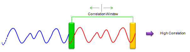
Aligned: the green window sits on the cyclic prefix, and the orange window sits on the end of the same symbol, so the two segments match.

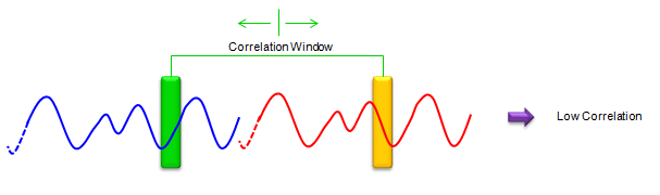
Misaligned: the two windows cover unrelated parts of the signal, so the correlation stays low.

• The two windows are one FFT length apart : the green one on the cyclic prefix, the orange one at the end of the symbol.
• High correlation marks the cyclic prefix : and the symbol starts right after it.
• No reference signal is needed : the method uses only the structure of the OFDM symbol.
• The floor between peaks is noisy : so the method gives a rough timing estimate, as the text above says.

The correlation carries more than timing. r is a complex number, and its phase shows how much the signal rotated over one FFT length. A carrier frequency offset adds to that rotation, so the phase at the peaks can also give a rough frequency estimate. The drawings also assume that the cyclic prefix is an exact copy, which holds for the LTE downlink but not quite for the uplink, as the two results below show.

Matlab Code

The method needs only two numbers from the signal: the FFT length, which sets the lag between the two windows, and the cyclic prefix length, which sets the window size. The code below takes both from the LTE numerology.

Following is a sample Matlab code to calcualting correlation with the length of cyclic prefix sliding along the I/Q data sequence.

clear all;

 

 

fid = fopen('UL_5_25_NoFilter_S7_68_Trig.bin','r');

[data,count] = fread(fid, 'single');

fclose(fid);

 

Offset = 280228 + 2 ;

 

Nfft = 512;

SamplingScale = (double(Nfft)/2048);

CP_LengthList = SamplingScale * [160;144;144;144;144;144;144];

Symbol_LengthList = SamplingScale * [2048;2048;2048;2048;2048;2048;2048];

 

dataI = data(1:2:end);

dataQ = data(2:2:end);

dataComplex = dataI + j*dataQ;

 

rSeq = [];

rThreshold = 0.2;

rPeakIndex = [];

NoOfSymbolsToScan = 10;

 

SearchStart = 0;

 

for i = (SearchStart+0):(SearchStart + NoOfSymbolsToScan*Nfft + NoOfSymbolsToScan*144)

    X = dataComplex(i+1:i+144/4);

    Y = dataComplex(i+1+Nfft:i+Nfft+144/4);

    r = X' * Y;

    rSeq = [rSeq r];

end;

 

pks = find(abs(rSeq) > 0.24);

 

subplot(3,1,1);

plot(abs(rSeq),'r-'); xlim([1 length(rSeq)]); ylabel('r');

 

subplot(3,1,2);

plot(real(rSeq),'r-'); xlim([1 length(rSeq)]);ylabel('Re(r)');

 

subplot(3,1,3);

plot(imag(rSeq),'r-'); xlim([1 length(rSeq)]);ylabel('Im(r)');

 

 

The numbers in the code come from a 5 MHz LTE signal. N_fft = 512 gives a sampling rate of 7.68 Msps, a quarter of the 30.72 Msps reference, so SamplingScale is 0.25. The normal cyclic prefix of 144 T_s becomes 36 samples, and 160 T_s becomes 40. 36.211 v19.3.0 gives the same two lengths for the downlink in clause 6.12 and for the uplink in clause 5.6.

The loop compares a window X of 144/4 = 36 samples with the window Y that starts N_fft = 512 samples later, and stores r = X'Y. The window length ignores the longer first cyclic prefix of each slot, which is a simplification that the plots below tolerate. Two variables are set but never used: Offset, and rThreshold, because the peak search uses 0.24 instead.

• N_fft = 512 : 7.68 Msps, a 5 MHz LTE carrier.
• Window of 36 samples : the 144 T_s cyclic prefix at this sampling rate.
• Lag of 512 samples : the distance between the cyclic prefix and its copy.
• r = X'Y is complex : the plots show its magnitude, its real part and its imaginary part.

Result : Uplink IQ Data

The first data set is an uplink capture. The plot below shows |r|, Re(r) and Im(r) for about ten SC-FDMA symbols, and each sharp peak marks one cyclic prefix.

From an uplink IQ sample data (fid = fopen('UL_5_25_NoFilter_S7_68_Trig.bin','r') ), I got following result. (If you want to try this code with the same data that I used, download the data from the link)

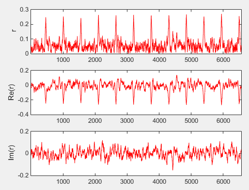
The peaks of |r| repeat about every 550 samples. Re(r) dips negative at every peak, while Im(r) shows no clear pattern.

• Peak spacing of about 550 samples : 512 samples of symbol plus about 36 samples of cyclic prefix.
• Re(r) is negative at the peaks : the uplink cyclic prefix is an inverted copy, as explained below.
• Im(r) stays near zero : the correlation phase is close to 180 degrees.

The negative real part is not noise. The LTE uplink shifts every subcarrier by half a subcarrier spacing, through the (k + 1/2)Δf term of 36.211 clause 5.6. Over one FFT length, 1/Δf, that shift turns the phase of every subcarrier by exactly π. So the uplink signal one FFT length after the cyclic prefix is the negative of the cyclic prefix, and r = X'Y comes out real and negative.

The downloadable file on this page has a different name from the one in the code. The link text says UL_5_25_NoFilter_S7_68_Trig.bin, but the file behind it is LTE_UL_5_1_CID_0_1RB_NoFilter.bin, so change the fopen() argument to match before running the code.

Result : Downlink IQ Data

The second data set is a downlink capture of a 5 MHz carrier with 25 RB. The same code runs on it unchanged, so any difference between the two plots comes from the signal, not from the method.

From a downlink IQ sample data (fid = fopen('LTE_DL_5M_25RB_S_7_68_SG_Trig.bin','r')), I got following result. (If you want to try this code with the same data that I used, download the data from the link)

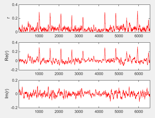
The peaks of |r| repeat at the same spacing as in the uplink. This time Re(r) is positive at every peak.

• Same peak spacing : one peak per OFDM symbol, about 550 samples apart.
• Re(r) is positive at the peaks : the downlink cyclic prefix is a true copy of the end of the symbol.
• One peak is missing near sample 3750 : the correlation there stays below the others in this capture.

The positive sign follows from the downlink formula. 36.211 clause 6.12 uses kΔf without the half-subcarrier shift and leaves the DC subcarrier empty instead. Every subcarrier then turns a whole number of cycles over one FFT length, so the cyclic prefix is an exact copy and r is real and positive. Comparing the sign of Re(r) at the peaks is therefore a quick way to tell an LTE uplink capture from a downlink one.

• Uplink: Re(r) negative : half-subcarrier shift, inverted copy.
• Downlink: Re(r) positive : no shift, exact copy.
• A residual frequency offset rotates r : a phase away from 0 or 180 degrees points to a frequency error.

Reference

[1] 3GPP TS 36.211 v19.3.0 - clause 5.6 for SC-FDMA and clause 6.12 for OFDM baseband signal generation

[2] OFDM : Cyclic Prefix