comm.OFDMModulator turns a column of frequency domain values into a time domain waveform, and its defaults already describe a complete OFDM symbol. This page creates the object and reads back what the defaults decided. It then rebuilds the same output by hand, so that nothing inside step() stays hidden.

• Creating OFDM Modulator
• What do the default properties control ?
• Generating OFDM Symbol Data with Default Setting
• Generating OFDM Symbol Data with Internal Procedure
• Where do these defaults come from ?
• What does this example leave out ?

Creating OFDM Modulator

Two lines create the object and read back what it decided for you. The constructor takes no required arguments, so every property in the first table below is a default rather than a choice. The info() call reports the two sizes those defaults imply.

hMod = comm.OFDMModulator;

hModInfo = info(hMod);

 

hMod

Properties:                FFTLength: 64        NumGuardBandCarriers: [6;5]             InsertDCNull: false           PilotInputPort: false       CyclicPrefixLength: 16                   Windowing: false               NumSymbols: 1          NumTransmitAntennas: 1

 

hModInfo

DataInputSize: [53 1]       OutputSize: [80 1]

FFTLength = NumGuardBandCarriers(1) + DataInputSize +  NumGuardBandCarriers(2) = 6 + 53 + 5 = 64

OutputSize = FFTLength + CyclicPrefixLength = 64 + 16 = 80

Read those two lines in the right direction. DataInputSize is not a setting, and neither is OutputSize. You choose FFTLength, the two guard band sizes and the cyclic prefix length. Matlab then works out how many values it needs from you, and how many samples it will return. That is the whole reason info() exists as a separate call.

The consequence matters as soon as you change anything. Raise FFTLength, widen a guard band or turn on the DC null, and DataInputSize changes with it. Code that hard-codes 53 breaks silently at that point, which is why the example below builds its input from hModInfo.DataInputSize rather than from a literal.

Figure 1 puts both equations in one picture, with the frequency domain array above and the time domain output below.

Figure 1. The two equations drawn to scale. The guard bands are positions in the array rather than values you supply, and the cyclic prefix is a copy rather than new information. The 53 numbers you provide are therefore the only information in the 80 samples.

• The blue block is the only place your data goes : the object fills the grey blocks with zeros. The orange block is a copy of the blue block's tail, taken after the transform.
• The two rows are not in the same units : the upper bar is one entry per subcarrier position, and the lower bar is one entry per time sample. They share a length of 64 only because an N point IFFT returns N samples.
• 80 samples carry 53 numbers : the extra length buys spectral shaping at the band edges and tolerance of delay spread. It costs the difference in throughput.

What do the default properties control ?

Matlab prints that property list and explains none of it, so here is what each line does. Four of the eight decide how many values you have to supply. Two change the shape of that input, and the last two touch only the output waveform.

The table has one pattern behind it. Anything that removes a position from the payload also removes a row from DataInputSize. Guard bands, a DC null and a pilot port therefore all shrink the input you have to build. Anything that lengthens the waveform in time moves OutputSize instead. FFTLength is the only property that moves both, because it fixes the payload and the symbol length together.

That pattern is also the argument for calling info(). Read the property values and do the subtraction yourself, and that works until you enable the pilot port. From that point the answer depends on how many pilot positions you asked for. The object already knows the number, so ask it rather than recompute it.

• Four properties change how much data you must supply : FFTLength, NumGuardBandCarriers, InsertDCNull and PilotInputPort all move DataInputSize. NumSymbols and NumTransmitAntennas change its shape, and the remaining two touch only the output.
• Calling info() is not a convenience : DataInputSize and OutputSize are derived rather than set. Reading them back is the only way to stay correct after a property changes.
• Two defaults are switched off rather than missing : Windowing and PilotInputPort exist on the object and are false. What follows is therefore a plain OFDM chain rather than a complete transmitter.

Generating OFDM Symbol Data with Default Setting

The first run drives the object with random complex values and plots the magnitude at each end. A plot is the quickest way to confirm the two sizes computed above. It also exposes a change of scale that catches most people comparing the two panels.

hMod = comm.OFDMModulator;

hModInfo = info(hMod);

 

rng(0);

dataIn = complex(randn(hModInfo.DataInputSize),randn(hModInfo.DataInputSize));

modData = step(hMod,dataIn);

 

subplot(2,1,1);

stem(abs(dataIn));xlim([1 length(dataIn)]);title('Input Data');

subplot(2,1,2);

stem(abs(modData));xlim([1 length(modData)]); title('Output Data');

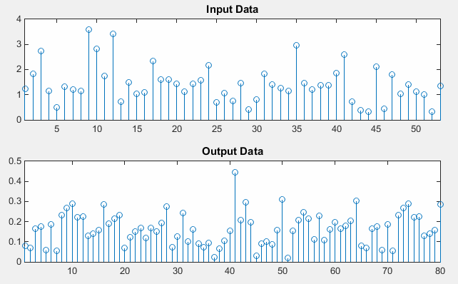
Figure 2. The two sizes from info() drawn as x-axis limits : 53 in, 80 out. The vertical scales are not the same, so the two panels cannot be compared by eye without reading each axis first.

• The x-axis carries the result : the upper panel runs to 53 and the lower panel runs to 80. Those are DataInputSize and OutputSize, taken straight from the table above.
• The y-axes disagree by a factor near eight : the tallest input stem reaches about 3.6 and the tallest output stem about 0.44. Matlab rescales every axis on its own, so the output looks flat until you read the numbers.
• Only magnitude is drawn : both panels plot abs(), and the values are complex on both sides. Half of what the modulator produced does not appear in either panel.

The change of scale has a cause worth knowing, because it appears every time you plot an IFFT output. Matlab's ifft includes the 1 over FFTLength factor, so it divides by 64 while summing 53 contributions that are independent of each other. The output is therefore smaller in RMS by roughly 64 divided by the square root of 53, which is close to nine. The peaks in the two panels differ by about eight.

The practical version is short. An IFFT does not normalise its output to the input level, so a transmitter has to scale the waveform before it reaches a power amplifier. The figure shows the raw output, and nothing in the default settings adjusts it.

• Build the input from hModInfo, never from 53 : the example writes randn(hModInfo.DataInputSize) for exactly this reason, so the line still works after a change of FFTLength.
• Fixing the seed is what makes the picture repeatable : the data is random, and rng(0) produces the same draw every run. That is the only reason your plot can be compared against this one.
• The amplitude drop is arithmetic, not loss : no energy disappears in the IFFT. The 1 over N factor in Matlab's definition is a convention, and the scaling a transmitter needs is a separate decision.

Generating OFDM Symbol Data with Internal Procedure

The second run replaces step() with the three operations it performs, and then calls step() as well so that both results appear in one figure. Everything rests on the bottom two panels, which have to match if the manual chain is complete.

hMod = comm.OFDMModulator;

hModInfo = info(hMod);

 

rng(0);

dataIn = complex(randn(hModInfo.DataInputSize),randn(hModInfo.DataInputSize));

dataInGuardBand = [zeros(hMod.NumGuardBandCarriers(1),1); ...

                           dataIn; ...

                           zeros(hMod.NumGuardBandCarriers(2),1)];

dataInGuardBandIfft = ifft(dataInGuardBand);

CP = dataInGuardBandIfft(length(dataInGuardBandIfft)-(hMod.CyclicPrefixLength)+1: ...

                                   length(dataInGuardBandIfft));

dataInGuardBandIfftCP = [CP ; dataInGuardBandIfft];

 

modData = step(hMod,dataIn);

 

subplot(5,1,1);

stem(abs(dataIn));xlim([1 length(dataIn)]);title('Input Data');

subplot(5,1,2);

stem(abs(dataInGuardBand));xlim([1 length(dataInGuardBand)]);title('Input Data + GuardBand');

subplot(5,1,3);

stem(abs(dataInGuardBandIfft ));xlim([1 length(dataInGuardBandIfft)]);title('IFFT(Input Data + GuardBand)');

subplot(5,1,4);

stem(abs(dataInGuardBandIfftCP ));xlim([1 length(dataInGuardBandIfftCP)]);title('CP + IFFT(Input Data + GuardBand)');

subplot(5,1,5);

stem(abs(modData));xlim([1 length(modData)]); title('Output Data');

 



 

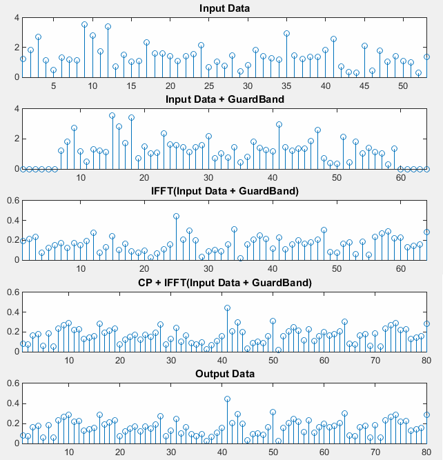
Figure 3. The chain drawn one stage at a time, with step() repeated at the bottom for comparison. The bottom two panels are the same picture, so for these default settings step() performs these three operations and nothing else.

• Panel 2 draws the guard bands instead of quoting them : it runs to 64, and its first six and last five stems sit flat on zero. That is NumGuardBandCarriers = [6;5] made visible.
• The tallest stem moves six places to the right : it sits near index 9 in panel 1 and near index 15 in panel 2. Six zeros were placed in front of it, and nothing else about the pattern changes.
• The vertical scale changes at the IFFT and nowhere else : panels 1 and 2 run to 4, and panels 3, 4 and 5 run to 0.6. Inserting zeros does not alter amplitude, and neither does copying a prefix.
• Panels 4 and 5 match : the hand built waveform and the step() output are the same, which is the result the whole section exists to demonstrate.

That last point is the important one, and it is worth stating as a negative. For these default settings step() applies no extra scaling, no windowing and no reordering of the subcarriers before the transform. A plain ifft on the zero padded column reproduces it exactly. Anything else you might expect from a real transmitter is absent here because the property that would add it is switched off.

Look closely at the cyclic prefix line. It slices the last CyclicPrefixLength samples out of the IFFT output and places that copy in front. The waveform therefore starts partway through the symbol and then runs through the whole of it. A receiver can therefore begin its 64 sample window anywhere in the first 16 samples and still capture one complete period. That tolerance is what the prefix buys with its 20 per cent of the symbol.

• The prefix is a copy of the tail, not padding : the code takes the last 16 samples rather than 16 zeros. That choice is what lets a delayed copy of the signal still look periodic to the receiver.
• Three lines replace one object : zero padding, ifft and a slice. Reading them once removes any mystery from step().
• 16 out of 80 samples carry nothing new : a fifth of the symbol goes to the prefix. That is the price of the delay tolerance it provides.

Where do these defaults come from ?

Those defaults look oddly specific. Why a 64 point FFT, why guard bands of 6 and 5, and why exactly 16 samples of cyclic prefix ? They are the OFDM symbol of 802.11a, and recognising that explains the whole property list at once.

The table below sets the two side by side. Wi-Fi at 20 MHz uses a 64 point FFT with subcarriers numbered from minus 26 to plus 26. That leaves the six most negative and the five most positive positions empty. Its cyclic prefix is 0.8 microseconds of a 4 microsecond symbol, and at 20 MHz that is 16 samples.

The last two rows are where the toolbox default and the standard differ. 802.11a leaves the centre subcarrier empty and spends four more on pilots, so 52 positions are occupied and only 48 of them carry payload. Setting InsertDCNull to true and PilotInputPort to true makes the object match the standard on both counts, and DataInputSize drops as each one is enabled.

A cellular numerology is much further away, and it is worth knowing how far. LTE at 20 MHz uses a 2048 point FFT with 1200 active subcarriers. FFTLength and both guard band sizes therefore change by a factor of more than thirty. Its cyclic prefix is longer in samples than this one, and the first symbol of each slot carries a longer prefix than the rest. A single CyclicPrefixLength value therefore cannot describe a whole slot. NR keeps the same construction and makes the subcarrier spacing selectable. The object handles all of it, and none of it is what you get by typing comm.OFDMModulator with no arguments.

• The defaults are a Wi-Fi symbol, not a neutral starting point : 64, [6;5] and 16 all come from 802.11a. The object begins as a description of a real system rather than an abstract one.
• 53 is not 48 : the default leaves DC occupied and reserves nothing for pilots, so the payload is five values larger than a Wi-Fi symbol carries.
• A cellular symbol needs every property changed : LTE and NR use a much larger FFT, much wider guard bands and a prefix that varies within a slot. Treating these defaults as typical will mislead you.

What does this example leave out ?

The example above is complete as an OFDM modulator and incomplete as a transmitter. Knowing which pieces are missing matters, because each missing piece is the reason some later result fails to match a standard.

Start with the input itself. The variable dataIn is complex(randn, randn), which is Gaussian noise rather than a constellation. That is why the input stems in Figure 2 spread over a continuous range of magnitudes instead of landing on a few fixed levels. A real chain puts a QAM or PSK modulator in front, and every value entering the OFDM modulator is then one point of a constellation.

The object itself is running at its smallest setting in three ways. NumSymbols is 1, so the output holds a single symbol and there is no boundary between symbols anywhere in it. Windowing therefore has nothing to smooth, which is why leaving it false costs nothing here and costs a great deal in a real transmitter. NumTransmitAntennas is 1, so there is no spatial dimension and no precoding.

Two omissions matter at the far end rather than this one. The waveform carries no pilots, so the receiver has no known values to estimate the channel from. It can only be demodulated through a channel that leaves it unchanged. Without a DC null the centre subcarrier carries data, and a direct conversion receiver puts its own DC offset in exactly that bin. Both are properties rather than missing features, and each can be enabled with one line.

The other half of this page is the receive side. OFDM DeModulator reverses these same three operations, and OFDM Details goes further into the properties. For the theory behind the transform rather than the toolbox call, OFDM covers the subject on its own.

• The input is noise, not a constellation : randn produces a continuous spread of magnitudes. That is why the upper panel of Figure 2 looks nothing like the output of a QAM mapper.
• One symbol hides the cost of Windowing : the output holds no symbol boundary, so the property that would smooth one has nothing to act on and no visible price.
• No pilots means no channel estimation : the waveform is complete, and a receiver still needs known values somewhere in it before a real channel can be undone.
• Every gap here is a property, not a limitation : pilots, DC null, windowing, multiple symbols and multiple antennas are all supported. Each one changes DataInputSize or its shape, so read info() again after each change.