Spread Spectrum in Wireless Communication refers to a technology to spread narrow spectrum data (low chip rate) to wider spectrum (high chip rate). This technique has been used in early WLAN (e.g, 802.11b), CDMA, WCDMA.

• How the spreading works
• Spreading factor and chip rate
• What the spectra do and do not show
• Why Spreading ?
• Spreading, channelization and scrambling
• Octave Script
• Reference

How the spreading works

Spreading buys something by giving away bandwidth, and the trade only makes sense once the something is named. The figure below runs one data sequence through the whole operation and back again, so the cost in bandwidth and the shape of the recovery are both on the page before any reason for paying it arrives.

A typical method of spreading a spectrum is illustrated as below.

[1] - this indicates the original data. This is assumed to be relatively low chip rate.

[2] - this indicates the frequence response of the data ([1]). As you see here, the frequency waveform looks very narrow.

[3] - this indicate a specific sequence of chips called 'spreading code'. Intuitively, you would notice that this has higher chip rate than the data.

[4] - this indicates the frequency response of the spreading code([3]). Intuitively, you would notice that this has much wider bandwidth in spectrum.

[5] - this shows the result of applying XOR to data sequence and spreading code sequence. This process is called 'spreading'. By this step, the data of low chip rate is converted to another sequence with higher chip rate.

[6] - this indicate the frequency response of the sequence [5]. This shows the much wider frequency band comparing to the data spectrum ([2]).

[7] - This is to show how to convert the spreaded sequence to the original data sequence. The method is very simple. Just XOR the spreaded sequence with the same spreading sequence and it gives you the original sequence.

[8] - this indicates the frequency response of the sequence [7].

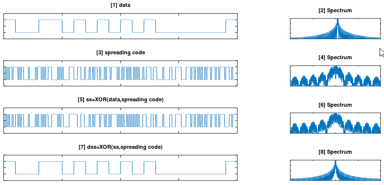
Figure 1. One sequence spread and then recovered, with the spectrum of every stage beside it. The left column is time and the right column is frequency, and the interesting comparison runs down each column rather than across.

• The top and bottom rows are the same signal : panel [7] reproduces panel [1] sample for sample, and panel [8] reproduces the narrow shape of panel [2]. The spectrum goes out wide and comes back.
• Panel [5] looks like panel [3] rather than like panel [1] : the spread signal carries the data and shows none of it. That is the whole effect, and the section below explains why the data is still in there.
• Panels [4] and [6] are the same width : spreading pushes the occupied band out to the width the code already had, and no further. The code sets the bandwidth, and the data does not.
• The wide spectra show several lobes : each is the transform of a rectangular chip, so a main lobe sits in the middle with sidelobes either side. The narrow spectra in [2] and [8] have the same shape ten times compressed.
• Every spectrum is drawn in dB against its own peak : the script divides each one by its maximum before plotting, so all four reach the top of their axis. The picture therefore compares shapes and cannot compare levels.

The arithmetic behind the picture is in the script at the foot of the page. It builds 20 data bits and 200 code chips over the same 2000 samples, so one data bit covers exactly 10 chips. That ratio of 10 is what the next section calls the spreading factor.

Spreading itself is one XOR per sample. Map a 0 to +1 and a 1 to -1, and XOR becomes multiplication, so the spread signal is the data multiplied by the code. A data bit of 0 therefore sends the code unchanged, and a data bit of 1 sends the code inverted. Panel [5] looks like panel [3] because it is the code, with the sign flipped over the stretches where the data is 1.

Recovery needs no new operation. XOR is its own inverse, so applying the same code a second time cancels it and returns the data, which is what the script does to produce panel [7] and what the author's note under [7] describes. Nothing has to be inverted and nothing is estimated.

One condition is implied and never stated. The receiver must apply the same code at the same chip position, because a code shifted by one chip cancels nothing. Getting that alignment is the acquisition problem, and it is the work that a spread spectrum receiver does before any data comes out.

• XOR with the code is multiplication by plus or minus one : the data chooses between the code and its inverse, which is why the spread signal inherits the code's rate and the code's spectrum.
• One data bit covers ten chips here : 20 bits and 200 chips share 2000 samples in the script, and that ratio governs everything else on this page.
• Despreading is the same operation again : the code enters twice and cancels, so transmitter and receiver run identical hardware.
• Chip alignment is assumed, not given : a one chip offset destroys the cancellation, so a real receiver has to acquire the code phase first.

Spreading factor and chip rate

The three notes below fix the numbers the rest of this page depends on, and each of them names a chip rate. A chip rate on its own settles nothing, because what a reader wants is the data rate underneath it. The spreading factor is what connects the two, and the division is done after the notes.

NOTE 1 : As shown in Figure 1, you would notice that the chip rate of the scrambled data gets higher than the chip rate of the original data. The ratio of the original data chip rate and the spreaded chip rate is called Spreading Factor.

NOTE 2 : In CDMA, a set of specially designed spreading code called Walsh code are used to spread the data in such a way that the chip rate of the spreaded data become 1.2288 Mcps (Mega chips per second). In Walsh Code, every spreading code has same spreading factor.

NOTE 3 : In WCDMA, a set of specially designed spreading code called OVSF(Orthogonal Variable Spreading Factor) code are used to spread the data in such a way that the chip rate of the spreaded data become 3.84 Mcps (Mega chips per second). In OVSF, there are multiple levels of code sets with different spreading factors. Depending on the data rate to be achieved, different spreading factors are applied.

Those three notes carry one piece of arithmetic between them and never write it down. The chip rate divided by the spreading factor is the symbol rate, so the spreading factor is what turns a fixed number of chips per second into a variable number of symbols per second. Everything a designer chooses sits in that division.

The CDMA case in NOTE 2 is the simple one. A Walsh code of length 64 against a chip rate of 1.2288 Mcps gives 19.2 ksymbols per second, and because every Walsh code in the set has the same length, every channel gets the same rate. One chip rate and one spreading factor leave nothing to decide.

The WCDMA case in NOTE 3 is where the variable in OVSF earns its name. The chip rate stays at 3.84 Mcps whatever happens, and the spreading factor moves in powers of two, so the symbol rate moves with it. The table below does the division.

• The chip rate never changes : a WCDMA transmitter runs at 3.84 Mcps for a 7.5 ksps channel and for a 960 ksps channel alike, which is what lets one radio carry both.
• A lower spreading factor buys rate and costs protection : the two right hand columns move in opposite directions, and choosing a spreading factor is choosing a point on that trade.
• The processing gain column is the reason the trade is not free : it is ten times the logarithm of the spreading factor, and the section after next says what those decibels do.
• The figure uses a spreading factor of 10 : that is not an OVSF value, since OVSF factors are powers of two. It is chosen to make the picture readable, which is the caveat the author gives above the script.

What the spectra do and do not show

Four spectra sit in Figure 1 and every one of them reaches the top of its axis. That is an artefact of how they are drawn, not a property of the signals, and the difference it hides is the one that matters. Reading the figure without knowing this leads to the wrong conclusion about what spreading costs.

The script normalises before it plots. Each spectrum is divided by its own maximum and then converted to dB, so every curve peaks at 0 dB by construction and the vertical axis runs from there down to -40 dB. Shapes can be compared across the four panels, and levels cannot.

The levels are not equal, and the reason is that spreading adds no power. Every sample of the data trace and every sample of the spread trace is plus or minus one, so the sum of squares over the 2000 samples is 2000 in both cases. The same power now occupies ten times the bandwidth, so the power in any given slice of spectrum has fallen by a factor of ten.

Ten times is 10 dB, and the general form is ten times the logarithm of the spreading factor. An averaged periodogram of the two signals puts the drop in peak spectral density at 9.87 dB against the 10.00 dB the arithmetic predicts. Figure 2 redraws the pair with that level restored.

Figure 2. The same pair of spectra drawn twice. On the left each curve is divided by its own peak, which is what Figure 1 does and what makes the two look equally tall. On the right they keep the level the transmitter gives them, and the spread one sits 10 dB lower across a band ten times as wide.

• The left panel is Figure 1 and the right panel is the radio : the normalisation is a plotting convenience, and the 10 dB step on the right is what a spectrum analyser would measure.
• The area under the two curves is the same : the wide one is ten times broader and 10 dB lower, and those two factors cancel. Spreading redistributes power and never creates or destroys it.
• The first null moves out by the spreading factor : the narrow curve nulls at the data rate and the wide one at the chip rate, ten times further out.
• The sidelobe pattern is identical in both : the same rectangular pulse shape produces it, stretched along the frequency axis.

A signal whose power spectral density has dropped by 10 dB can fall below the noise floor of a receiver that looks at a narrow slice of the band. The total power has not changed, so the wanted receiver still collects all of it by gathering the whole band and despreading. An observer without the code sees a slightly raised noise floor and nothing else.

The same property lets a spread signal share a band with narrowband users without raising their noise by much. The interference it adds to any one narrow channel is a tenth of its total power here, and a far smaller fraction at the spreading factors of 64 or 256 that real systems use. The next section covers what despreading does to interference arriving the other way.

Why Spreading ?

Why we do spread spreading ? There can be several advantages coming out of this technology. With specially designed spreading code, we can achieve advantages as follows.

• We can make the chip rate of the signal at physical layer all the same regardless of chip rate (data rate) of user data
• We can make the user data a random-like data which would make unwanted deciphering very difficult (i.e, improving security)
• We can use scrambling codes as a tool to differetiate various physical channels occupying the same spectrum as other channels. When a scrambling code is used for this purpose, they are often called as 'channelization code'.

One reason is missing from that list, and it is the reason spread spectrum was invented rather than a convenience that came with it. Spreading buys resistance to interference, and the amount it buys is the spreading factor. Expressed in decibels it is called the processing gain, and for the factor of 10 in Figure 1 it is 10 dB.

The mechanism is an asymmetry in how often the code is applied. The wanted signal meets the code twice, once at the transmitter and once at the receiver, so the two cancel and the signal collapses back to the data bandwidth. Anything else on the air meets the code only once, at the receiver, so it gets spread rather than collapsed.

What follows is a filter matched to the data bandwidth. All of the wanted signal is inside it, and only the fraction of the interferer that landed in that narrow slice survives. That fraction is one over the spreading factor. Figure 3 follows a narrowband interferer through the three stages.

Figure 3. Why the code is applied twice to the signal and once to everything else. Despreading collapses the wanted signal back into the data bandwidth and spreads the interferer across the chip bandwidth, after which the data filter keeps all of the first and a tenth of the second.

• Panels 2 and 3 are the same two signals with their shapes exchanged : the interferer starts ten times taller than the signal and ends ten times shorter. Nothing was amplified, and only the bandwidths changed.
• The code is what makes the two behave differently : the signal carries it already and the interferer does not, so one multiplication undoes it for the first and imposes it on the second.
• The dashed box is where the gain is collected : without a filter narrow enough to reject the spread interferer, despreading on its own changes nothing.
• The interferer never has to be identified : no notch is tuned and nothing is measured, because the treatment falls out of the code the receiver was already applying.

The size of the effect is worth a number. A simulation with 10 chips per bit and a continuous wave interferer at a quarter of the chip rate, three times the signal amplitude, gives a signal to interference ratio of -6.5 dB before despreading and +3.5 dB after it. The difference is 10.0 dB, which is the processing gain.

At the spreading factors real systems use the figure is larger. A WCDMA channel at a spreading factor of 256 carries 24.1 dB of processing gain, which is why a signal sitting well below the interference on the air can still be received. The table in the spreading factor section above gives the rest.

The same arithmetic is what makes code division multiple access work, and it is the reason the first bullet above matters. Every other user in the cell is an interferer that arrives without this receiver's code, so each of them is spread by the despreading operation in exactly the way Figure 3 shows. The processing gain is the budget that pays for them, and the number of users a cell can carry is set by how much of it remains once the wanted signal has taken its share.

One entry in the list deserves a caution rather than an extension. The second bullet offers improved security, and a spreading code supplies very little of it, because the code sets used by CDMA and WCDMA are published in the specifications along with the rule for choosing between them. The pseudo random sequence page works through why a sequence of this kind resists an observer so poorly. What spreading genuinely gives an eavesdropper is a low power spectral density, which makes the signal hard to notice rather than hard to read.

• Processing gain is the entry the list is missing : ten times the logarithm of the spreading factor, which is 10 dB in Figure 1 and 24.1 dB at a spreading factor of 256.
• The gain comes from applying the code an odd number of times to everything else : the wanted signal sees it twice and cancels, and an interferer sees it once and spreads.
• A narrow filter after despreading is what collects the gain : measured at 10.0 dB for a continuous wave interferer at a spreading factor of 10.
• Other users are interferers like any other : the processing gain is the budget that multiple access spends, which is what turns this page into CDMA.
• Hard to notice is not hard to read : the codes are published, so the security in the second bullet is low probability of intercept rather than confidentiality.

Spreading, channelization and scrambling

This page uses three names around one operation, and they do not mean the same thing. A reader who has followed the figure now knows exactly one of them, and the other two belong to a second layer of coding that the figure never shows. Keeping them apart takes one table and one idea.

The idea is that orthogonality has a condition attached. A set of OVSF or Walsh codes gives exactly zero correlation between its members only when they are aligned chip for chip. One transmitter can guarantee that for its own channels, because it generates them from one clock. No transmitter can guarantee it against a different transmitter some distance away.

Two layers follow from that. The spreading code separates channels that share a clock, and it is the layer Figure 1 draws. A second code then separates transmitters that do not share one, and it cannot rely on orthogonality, so it uses long sequences with low cross-correlation instead. That second layer is the scrambling code.

• Only the left column changes the rate : that is the test that tells the two apart, and it is why only the left column appears in Figure 1.
• The right column is what lets the left column be reused : every cell can use the same small set of spreading codes, because the scrambling code underneath them differs.
• Orthogonal and uncorrelated are not the same guarantee : the first is exact and needs alignment, and the second is approximate and does not.
• A second layer costs no bandwidth : scrambling runs at the chip rate the spreading code has already set, so it adds separation without spreading anything further.

That leaves one thing to correct in the list above. The third bullet describes codes that separate physical channels sharing a spectrum, which is the job of the channelization code, and then gives that job to the scrambling code. The two names are the other way round. The site's own WCDMA scrambling code page puts it directly. The spreading code matches the bit rate to the 3.84 Mcps chip rate and separates one channel from another. Scrambling runs at that same chip rate and leaves it alone.

The distinction is worth the paragraph because the two layers fail differently. Exhaust the channelization codes and a cell cannot admit another channel, whatever its power budget. Give two cells the same scrambling code and their users collide no matter how many channelization codes are free. The scrambling code page carries the same comparison from the other side, with encryption added to it.

Octave Script

Following is the octave script that produced the plots show above. This is just for visualize the concept of spread spectrum, but not strictly complies to the implementation of spread spectrum in real world (e.g, CDMA, WCDMA, 802.11b)

Three details in that listing decide what the figure looks like, and the first is the one worth pausing on. Both N1 and N2 carry the comment Upsampling Rate, and they are not the same kind of quantity. N1 is 100 and stretches each data bit to 100 samples, while N2 is 10 and stretches each chip to 10.

The spreading factor is neither of those numbers. It is their ratio. Dividing 2000 samples by 100 gives 20 data bits and dividing by 10 gives 200 chips, so 10 chips cover each bit. Changing N1 alone therefore changes the spreading factor, and changing both together only changes how smooth the traces look.

The second detail is the seed, because rand("seed", 102) is set before either sequence is drawn. The figure above is therefore reproduced exactly rather than approximately. The third is the truncation. Convolving a 2000 sample array with a rectangle of length N returns 2000 plus N minus 1 samples. That makes sig1_pulse 2099 long and sig2_pulse 2009, so every later line writes (1:2000) to bring them back to a common length.

One thing the listing does that the plots do not advertise is the normalisation. Each spectrum is divided by its own maximum before the dB conversion, which is what the spectra section above is about. Deleting those four division lines would make the levels comparable and push three of the four traces off the bottom of a 40 dB axis.

• N1 and N2 are a ratio, not two settings : 100 over 10 is the spreading factor of 10, and only their ratio changes what the figure demonstrates.
• The seed makes the figure reproducible : anyone running the listing unchanged gets the panels printed above.
• (1:2000) is there because conv lengthens its input : the two pulse arrays come out 2099 and 2009 samples long and have to meet at 2000.
• The 4 by 3 grid is fully used : four wide traces span two cells each and four spectra take one cell each, which accounts for all twelve.
• The author's caveat above the listing is the right one : a spreading factor of 10 is not an OVSF value, and the script is drawn for legibility rather than for compliance.

Reference

[1] CDMA Overview

[2] Principles of DS-CDMA