Scrambling in communication usually indicates a process to convert a specific sequence to another sequence which is 'random-like' sequence. I am saying 'random-like', not 'random'. It mean it would just look like random, but it is generated by well defined deterministic way and the random-like sequence can be easily removed by a systematic way.

There are different ways for scrambling, but a common way is to generate a specific sequence called Scrambling Sequence and multiply (XOR in binary) it with the data that you want to scramble. As an example, you can see this type of scrambling in WCDMA Scrambling process.

• How does scrambling work ?
• Why Scrambling ?
• Why does the correlation have no peak ?
• Scrambling, spreading and encryption
• Octave Script
• Reference

How does scrambling work ?

A typical method of scrambling is illustrated as below. This is just to visualize the concept of scrambling process. It does not comply with any industrial specification (e.g, 3GPP).

[1] - This is the data that will be scrambled.

[2] - This is just to show that the first 10 % of the data [1], so that you can recognize the pattern more easily.

[3] - This is the sequence that will be used as a scrambler (i.e, scrambling code).

[4] - This is just to show that the first 10 % of the data [3], so that you can recognize the pattern more easily.  

[5] - This is the result of the sequence [1] that has been scrambled by the sequence [3].

[6] - This is just to show that the first 10 % of the data [5], so that you can recognize the pattern more easily.

[7] - This is the descrambled result of the sequence [5] using the scrambling code [3]

[8] - This is just to show that the first 10 % of the data [7], so that you can recognize the pattern more easily

[9] - This shows the result of cross correlation between the scrambled code [5] and the scrambling code [3]

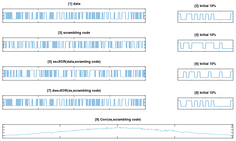
Figure 1. One scramble and one descramble, drawn end to end. Panels [1], [3], [5] and [7] run the full 2000 samples, and the narrow panels beside them repeat the first tenth so that individual bits are visible. The wide trace at the bottom is the correlation discussed further down this page.

• The left column is the whole record and the right column is a zoom : [2], [4], [6] and [8] plot the same sequences as [1], [3], [5] and [7], over the first 200 samples instead of all 2000. Nothing new is computed for them.
• Compare [2] against [8] rather than [1] against [7] : the two full length traces are too dense to read bit by bit. The two zooms are drawn at the same scale, so any difference between them would show. There is none.
• Panel [5] is the only one that looks different : the scrambled sequence has no long runs of a single level, while the data in [1] does. That change is the reason the whole operation exists.
• The title of panel [5] reads scramling code : the word is misspelled inside the picture, which is generated by the script further down. The corresponding title string in the script carries the same typo.
• Panel [9] is the one this page has to explain : it is a correlation and it shows a broad hump rather than a sharp spike. That is the correct result rather than a fault, and the section below works out why.

Two properties carry the whole operation, and the figure demonstrates both without naming either. The first is that XOR is its own inverse. Applying the same bit twice returns the original value, because a XOR b XOR b equals a for every a and b.

That single fact explains why panel [7] reproduces panel [1] exactly rather than approximately. The scrambler forms ss = data XOR code, and the descrambler forms ss XOR code, so the code enters twice and cancels. Nothing has to be inverted, and the transmitter and the receiver run the same operation with the same sequence.

The second property is what lets the same operation be written as arithmetic. Map a 0 to +1 and a 1 to -1, and XOR becomes ordinary multiplication, so ss = data x code sample by sample. The script plots with the opposite mapping, 2*sig-1, which turns XOR into minus the product. Both sequences carry that sign together, so it cancels in every product and changes nothing that follows.

One number in the script invites a misreading, and it is worth settling before the correlation section. Both sequences are upsampled by ten, and the ten is not a spreading factor. The script generates 200 data bits and 200 code bits, then stretches each bit into ten identical samples so that the traces draw as rectangles rather than as spikes. One code bit covers exactly one data bit.

The consequence is that scrambling leaves the rate alone. A 2000 sample scrambled sequence comes out of a 2000 sample data sequence, and the bandwidth the signal occupies is the bandwidth the data already occupied. Spreading is the operation that trades rate for something else, and the section below separates the two.

Both ends therefore need the same sequence and the same position within it. Advance the code by a single bit at the receiver and the cancellation fails, because each sample is then XORed against the wrong code bit. Roughly half the data bits come out wrong, which is the same as guessing, so a scrambled link that has lost its alignment fails outright rather than degrading.

• XOR is its own inverse : the same sequence and the same operation both scramble and descramble, which is why [7] matches [1] bit for bit rather than closely.
• The ten is drawing, not spreading : 200 data bits and 200 code bits are each stretched to 2000 samples so the plots show rectangles. The code runs at the data rate.
• Alignment matters as much as the sequence : a one bit slip in the code puts about half the output bits wrong, so there is no graceful degradation to observe.
• Nothing about the data is assumed : the cancellation holds for any data at all, which is what separates this from a coding scheme that relies on the input having some property.

Why Scrambling ?

Two answers follow below, and both of them describe what scrambling achieves on the air. A receiver designer would give a different one first, because the damage an unscrambled sequence does happens inside the receiver. Those reasons are added after the two bullets.

• One of the most popular reason for scrambling would be to make a given sequence like a random-like sequence. I said 'random-like', not 'real random'. The scrambled sequence should be able to be unscrambled by deterministic / systematic way.
• By designing a set of scramble code (scrambling sequence) in a specific way, you can use it as a specific identification code for each transmitter. For example, in WCDMA all the physical channel carrying user data from a specific cell is scrambled by a specific scrambling code and this scrambling code can be the identifier of the physical cell that is transmitting the specific user data.

The reason a receiver designer would give first is the run of identical bits. A payload of zeros produces long stretches with no transition, and so do an idle channel and a repeated frame. A receiver recovers its symbol clock from transitions. Take those away and the clock drifts, after which the sampling instant moves away from the centre of each symbol.

A long run also moves the average level of the signal away from centre. Receivers that slice against a running average then set their threshold in the wrong place, and the errors that follow have nothing to do with noise. Scrambling removes both problems at once by making a long run improbable.

The guarantee is stronger than improbable for the case that motivates it. When the input is constant, the scrambled output equals the code, so the code's own run structure bounds the output directly. One full period of an m sequence of n stages holds no run of ones longer than n, and no run of zeros longer than n minus 1. A degree 6 generator therefore caps an all-zero payload at six identical bits. For arbitrary data the bound becomes statistical rather than absolute.

The third reason is the spectrum. A repeating data pattern concentrates its energy at the frequency of the repetition, which appears as a line rather than as a spread. A line can breach an emission limit that the same average power spread evenly would pass. Scrambling flattens the spectrum without changing the average power.

The fourth reason only appears once there is more than one transmitter. Two cells that scramble with different sequences interfere with each other as noise, because neither sequence correlates with the other. Two cells sending the same unscrambled pattern interfere coherently instead, and a coherent interferer is far harder to tolerate than a noise-like one of the same power.

That last reason is where the author's second bullet leads. Both LTE and NR initialise the scrambling sequence from the cell identity together with the identity of the addressed device, so no two cells and no two devices in a cell run the same sequence. The NR pseudo random sequence page gives the per-channel initialisation, where PDSCH mixes the RNTI, the codeword index and a scrambling identity that falls back to the physical cell ID.

• Clock recovery is the first practical reason : a receiver locks to transitions, and a run of identical bits supplies none. Scrambling guarantees transitions whatever the payload contains.
• A long run also shifts the average level : a slicer referenced to a running average then puts its threshold in the wrong place, which produces errors with no noise involved.
• The run length bound is absolute only for constant input : a constant payload makes the output equal to the code, so a degree n m sequence caps the run at n. Arbitrary data gets a statistical guarantee instead.
• A repeating pattern makes a spectral line : the same average power spread evenly passes an emission mask that a line breaches, so flattening the spectrum is worth doing on its own.
• Different sequences turn coherent interference into noise : two cells scrambling differently do not correlate, which is why the sequence is initialised from the cell identity rather than fixed.

Why does the correlation have no peak ?

Panel [9] is the one panel in Figure 1 that looks like a mistake. A correlation is normally drawn to show a single sharp spike standing over a flat floor, which is how the m sequence and Gold code pages present it. This one has a broad hump and no spike anywhere in it. The trace is correct, and following the reason settles what correlation can and cannot recover from a scrambled signal.

Start with what the script correlates. The line reads sig_corr = xcorr(sig_ss,sig2_pulse), and sig_ss is the sequence drawn in panel [5] while sig2_pulse is the code drawn in panel [3]. Those two panels are the inputs to [9], and neither of them is panel [7].

Now look at the operation at zero lag, which is where a peak would sit. In the signed mapping the scrambled sequence is ss = d x c, so multiplying it by the code again gives ss x c = d x c x c. Every c x c term equals +1, so what the correlator accumulates at zero lag is the data itself, sample by sample. Figure 2 sets that out on sixteen chips.

Figure 2. The same sixteen chips carried through both operations, with 0 drawn as + and 1 as -. Row (d) shows that multiplying the scrambled sequence by the code returns the data exactly, and that adding the result gives zero rather than a peak. Row (e) is the correlation that does peak, and it contains no data.

• Row (d) is the descrambler and the correlator at once : the same products serve both. The descrambler keeps them as sixteen separate values, and the correlator adds them into one.
• Adding them is where the information goes : row (d) carries the data perfectly and its sum carries none of it, because balanced data has as many plus cells as minus cells.
• Row (e) is the peak that survives : correlating the code against itself leaves no data in the product, so nothing cancels and the sum reaches the sample count.
• The sixteen chips are chosen balanced on purpose : the data word has eight zeros and eight ones, so row (d) sums to exactly zero. A real data word lands near zero rather than on it.

The magnitude on the real record follows from the same reasoning. The correlator adds 200 signed data bits there, each contributing ten samples, so the total behaves like a random walk of 200 steps rather than like 200 aligned ones. Its typical size is ten times the square root of 200, which is about 141 against a full scale of 2000, or some seven per cent. A peak would be 2000.

The broad hump in panel [9] has a separate cause, and naming it stops it being mistaken for a weak peak. The script plots its traces in signed form but calls xcorr on the raw 0/1 arrays, and two sequences averaging about 0.5 each give every product an average of about 0.25. The number of overlapping samples falls linearly on either side of the centre, so those constant terms trace a triangle peaking near a quarter of 2000, which is 500. The hump measures the length of the overlap and nothing else.

The useful conclusion is that correlation locates the code rather than the data behind it. Acquisition and timing correlate a received signal against a locally generated copy of the code, which is row (e), and that is the operation with a peak in it. Descrambling multiplies sample by sample and keeps every product, which is row (d). Neither can stand in for the other, and panel [9] is the demonstration.

One case does restore a peak, and it explains why spreading looks different. Restrict the sum to a span over which the data does not change, and every product inside that span shares one sign, so the sum reaches full scale for the span and its sign is the data bit. Taking the 2000 samples ten at a time gives exactly that, 200 windows each reaching plus or minus ten. Panel [9] runs one sum across all 200 data bits, which is why they cancel.

• No peak is the right answer, not a broken plot : the zero lag value is the sum of the data, which sits near zero for any balanced payload.
• The hump measures the overlap, not a signal : xcorr is called on the 0/1 arrays, whose average product of 0.25 traces a triangle peaking at a quarter of the record length.
• Correlation finds codes and XOR undoes scrambling : the first serves acquisition and timing, the second recovers data, and they are not interchangeable.
• A peak returns as soon as the window shrinks : summing over one data bit reaches full scale and reports that bit, which is the correlation a spreading receiver performs.

Scrambling, spreading and encryption

Three operations combine data with a pseudo-random sequence, and this page has now touched all three without separating them. Figure 1 invites both of the usual confusions. Its tenfold upsampling looks like spreading, and the phrase random-like in the opening paragraph sounds like encryption. Neither reading is right, and the table below is the shortest way to keep them apart.

The second row is the one that settles the spreading question. Scrambling consumes one code bit per data bit, so the output has the same number of bits as the input and needs the same bandwidth. Spreading consumes several chips per data symbol, so the output is faster than the input and occupies more spectrum. The tenfold factor in the script changes neither, because it is applied to the data and to the code alike.

The third row settles the encryption question, and it settles it flatly. Every scrambling sequence in a cellular specification is published, along with the rule that sets its starting state, so any receiver can generate it and any eavesdropper can too. The operation is signal conditioning rather than protection, and the pseudo random sequence page works through why a linear generator offers nothing against an observer even when the sequence is not published.

The last row is the page's own example, and WCDMA happens to use both radio operations at once. The channelization code spreads, taking a channel from its bit rate up to 3.84 Mcps, and the scrambling code then runs at that same chip rate and leaves it alone. Two channels sharing one channelization code can still be separated if their scrambling codes differ, and that reuse is what the scrambling layer makes possible.

• The rate row separates the three fastest : spreading changes the rate and the other two do not, so a sequence that runs at the data rate is not spreading whatever else it does.
• A published sequence cannot protect anything : the specification gives both the generator and its initialisation, so scrambling is worth no security claim at all.
• The two radio operations apply in sequence rather than as alternatives : WCDMA spreads first and scrambles second, and the scrambling layer is what lets a finite set of channelization codes be reused across cells.
• Encryption sits above the radio : it is applied where the key lives, not in the physical layer, so it appears nowhere in Figure 1.

Octave Script

The listing below produces the whole of Figure 1 in one run, and it needs no toolbox beyond the Octave core. It falls into four parts. Two random bit sequences are generated and upsampled, the scramble and the descramble are computed, the correlation is taken, and fifteen subplot cells are filled in.

Three details in that listing are worth knowing before running it. The first is the seed, because rand("seed", 102) fixes both sequences. The figure above is therefore reproduced exactly rather than approximately. Changing that number changes every panel except the correlation, whose shape does not depend on which sequences were drawn.

The second is the truncation. Each sequence is zero stuffed to 2000 samples and then convolved with a ten sample rectangle. A convolution returns one sample fewer than the sum of its two lengths, so sig1_pulse and sig2_pulse come out 2009 long rather than 2000. Every later use writes (1:2000) to discard the tail, which is what keeps the XOR operands the same length.

The third is that four spectra are computed and none is plotted. The four variables sig1_pulse_fft, sig2_pulse_fft, sig_ss_fft and sig_ds_fft are each built with an fft and a circshift, and no subplot refers to any of them. They appear to be left over from a version of the figure that showed the spectra, and deleting the four pairs of lines changes nothing on screen.

• The seed is what makes the figure reproducible : rand("seed", 102) is set before either sequence is drawn, so anybody running the listing gets the same panels.
• (1:2000) is there because conv lengthens its input : the pulse arrays come out 2009 long, and XOR needs two operands of equal length.
• The four fft blocks are dead code : the spectra are computed and never plotted, so a reader looking for the frequency domain in Figure 1 will not find it.
• The 5 by 3 grid is fully used : the wide panels span two cells each and the correlation spans a whole row as [13 15], which accounts for all fifteen.

Reference

[1] CDMA Overview

[2] Principles of DS-CDMA