The most important component of signal representation is to understand the meaning of 'delta' fuction. Delta function in discrete signal can be illustrated as below. As you see, delta function is a special function which has '1' only at t = 0 and '0' at all other points. (In case of continuous signal, Delta function is defined as a function where the width of the function is infenitely small and the area under the function is 1).

• Reading the definition off the drawing
• Two different deltas share one symbol
• Building a whole sequence out of shifted deltas
• The sifting property
• Picking one sample out of a continuous signal
• The same operation on a discrete signal
• Properties worth remembering
• Why a true delta can never be transmitted

Reading the definition off the drawing

The paragraph above states the definition in words. The drawing below states the same thing twice over, once as a plot and once as a pair of conditions. Read the two halves against each other before going on.

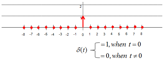
• The horizontal axis runs from -8 to 8 in integer steps, so the drawing is the discrete case. A red dot sits on the axis at every one of those indices.
• One red arrow rises at t = 0. It reaches the lower of the two dashed lines, which is height 1, and the upper dashed line marked 2 stays untouched.
• The definition at the lower right says the same thing in two lines : δ(t) = 1 when t = 0, and δ(t) = 0 when t is not 0.

The red dots are not decoration. Each one is the value 0 drawn at that index, so the plot carries seventeen values rather than one. Seventeen of them are zero, and exactly one is not.

The height of 1 is also a choice rather than an accident. It is what lets a delta be used as a multiplier further down this page, because multiplying by 1 leaves a value alone and multiplying by 0 removes it. A height of 2 would scale every result by 2.

One detail of notation is worth noting now, because the rest of the page leans on it. The symbol is written δ(t) with round brackets even though the axis is indexed by integers, and the sampling figures further down switch to square brackets for the discrete case.

Two different deltas share one symbol

The parenthesis in the opening paragraph gives a second definition without saying that it describes a different object. The discrete delta and the continuous delta are two different objects, and they share one symbol because they do the same job in their own settings.

The discrete one is an ordinary function, and the drawing above is exactly it. Its value is 1 at index 0 and 0 at every other index, so it can be written out as a list of numbers and stored in an array. Textbooks often call it the Kronecker delta.

The continuous one has no value at t = 0 at all. Its defining property is the area, as the opening paragraph says : the width shrinks towards zero while the height grows without limit, and the area stays 1. Nothing finite is left to plot, which is why every figure draws an arrow rather than a curve.

That object is not a function in the ordinary sense. Mathematicians call it a distribution, and it is defined by what it does inside an integral rather than by a value at a point. Writing δ(0) = infinity is a shorthand that no calculation ever uses.

The practical difference appears at the last step of a calculation. In the discrete case you multiply and read the answer straight off the result. In the continuous case you multiply and then integrate, and the integral is where the number appears.

One convention follows from that, and it explains a detail in the figures below. When an arrow is drawn for a continuous delta, its height on the page stands for the weight of the delta rather than for a value the signal reaches. The discrete case has no such gap, because there the height is the value.

Building a whole sequence out of shifted deltas

Why do we use this kind of special function ? It is because we can represent any discrete value by shift and multiplication of the function as shown below. (Note : In order for this kind of shift and multiplication to have practical meaning in real application, the system should be LTI (Linear Time Invariant). See Linearity and Time Invariance page.)

If you sum up all of these shift-multiplied versions of delta function, you can even express a sequence of signal in simple mathematical form.

If you want to express the following sequence without using the delta function, you may have to write s(t,x) = {(-8,0),(-7,2),(-6,0),(-5,0),(-4,1),(-3,0),(-2,0),(-1,0),(0,0),(1,0),(2,1),(3,0),(4,0),(5,2),(6,0),(7,0),(8,0)}. You would notice that it is simple to express it in the mathematical form.

Another reason why we use delta function for signal representation is the fact that the characteristics of the delta function is well investigated. Therefore, we can easily identify the characteristics of the signal based on the characteristics of the delta function. (Again, this holds true that the system is Linear Time Invarient).

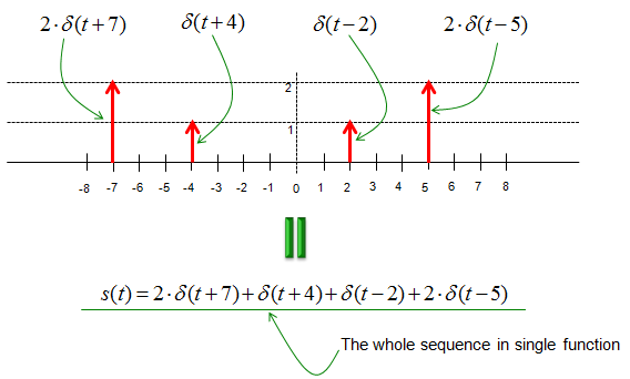
• The upper plot carries four red arrows. Two reach the upper dashed line at height 2, at t = -7 and at t = 5. The other two reach the lower dashed line at height 1, at t = -4 and at t = 2.
• Each arrow is labelled with the term that produces it. 2δ(t+7) and δ(t+4) sit to the left of the origin, and δ(t-2) and 2δ(t-5) sit to the right.
• The green equals sign leads down to one line, s(t) = 2δ(t+7) + δ(t+4) + δ(t-2) + 2δ(t-5), and the note beneath it calls that the whole sequence in single function.

The sign inside each bracket is the part most often read backwards. A plus shifts the arrow left and a minus shifts it right, because δ(t+7) is non-zero when t + 7 = 0, which happens at t = -7.

Each term therefore carries two numbers and nothing else. The coefficient in front sets the height, and the shift inside the bracket sets the position. One term is needed per non-zero sample, and no term is needed for the rest.

Compare that with the list written in the paragraph above. The list holds seventeen pairs, of which thirteen say that the signal is zero. The delta form writes down the four that are not, and that saving is the whole argument for using it.

The sifting property

Every figure from here on multiplies a signal by a shifted delta and then reads one number off the result. The rule that licenses that step has a name, and writing it down once saves explaining each figure on its own.

Take the discrete case first. Multiply x[t] by δ[t-k] term by term. Every term where t is not k gets multiplied by 0 and disappears, and the single term at t = k gets multiplied by 1 and survives. Summing over t therefore leaves x[k].

The continuous case says the same thing with an integral. The integral of x(t)δ(t-k) over all t is x(k). Here the delta has no value to multiply by, so the integral is what produces the number. The area of 1 is what makes the answer x(k) rather than some multiple of it.

The name for both statements is the sifting property, and some books call it the sampling property instead. The image behind the name is a sieve. Everything falls through except the one value at t = k.

One distinction matters before the figures below. The product x(t)δ(t-4) is still a function of t, and it is drawn as an arrow standing at t = 4. The sample x(4) is a number. The figures draw the product, and the number is the weight of the arrow that survives.

This rule is also what makes convolution work. An input written as a sum of shifted deltas passes through a linear time invariant system term by term, and the Convolution page continues from there.

Picking one sample out of a continuous signal

The delta function is also frequently used to represent 'sampling'. Let's say that we have a continuous signal x(t) and we want to express the value of x(t) sampled at t = 4. This can be respresented as shown below. I hope this make sense to you without any further explanation.

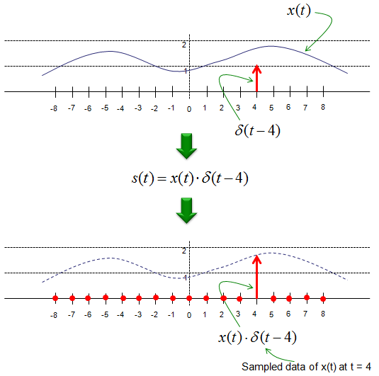
• The upper panel carries the continuous signal as a smooth curve with the label x(t) at its right, and a single red arrow standing at t = 4 labelled δ(t-4).
• The middle line states the operation, s(t) = x(t)δ(t-4), with a green arrow leading into it and another leading out.
• The lower panel redraws x(t) as a dashed curve and keeps one red arrow at t = 4. Red dots sit on the axis at every other marked position, so everything else is zero.
• The note at the bottom names the result : sampled data of x(t) at t = 4.

Read the two red arrows against each other. In the upper panel the arrow is δ(t-4) itself, so its weight is 1. In the lower panel the same arrow has been multiplied by x(4), so it now stands as high as the curve did at that instant.

That height is the answer the figure is after, and the section above says why it has to be read as a weight rather than as a value. The arrow is a continuous delta, so the signal does not reach that height anywhere. It is the number the sifting integral returns.

One sample is not yet sampling. Repeat this at every multiple of a fixed interval, and the single arrow becomes an impulse train, and the whole of Sampling Theory is built on what that train does to the spectrum.

The same operation on a discrete signal

This way of representing the sampling with delta function is also applies to the discrete signal as shown below. Let's say we have a discrete signal x[t] and you want to select out the value at index 4. You can just express it as below.

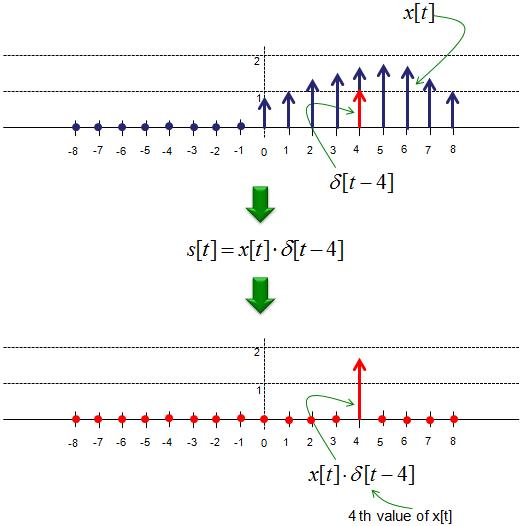
• The upper panel is a stem plot of x[t]. The samples from -8 to -1 are zero and drawn as dots on the axis, and blue arrows of varying height stand at the indices from 0 to 8.
• One arrow at index 4 is drawn red rather than blue and labelled δ[t-4], which marks the index being selected.
• The middle line states the operation in square brackets, s[t] = x[t]δ[t-4].
• The lower panel keeps a single red arrow at index 4 and puts dots on the axis everywhere else. The note calls that arrow the 4 th value of x[t].

The figure above writes the operation in square brackets, where the continuous version used round ones. Square brackets mark a discrete index and round brackets mark continuous time, which is the usual signal processing convention rather than anything specific to this page.

No integral is needed here, and that is the practical payoff of the discrete case. Multiplying term by term already leaves one non-zero entry, so the answer can be read straight off the lower plot without any further step.

The note at the bottom calls the survivor the 4 th value. That is the index rather than the position in the list. The indices start at 0, so the entry at index 4 is the fifth one counted from the start of the non-zero run.

This kind of mathematical expression may look unnecessarily complicated, but as I mentioned above if you can express your signal into this kind of mathematical form you can easily characterize your signal based on a simple well known signal (delta function). One common example for this is for investigation of the system output for a given input sequence.

Properties worth remembering

Five rules cover almost everything the delta function is used for, and two of them have already appeared in the figures above. Collecting them in one place makes the other three easier to put down.

The convolution identity is the reason a delta is called a unit impulse. Convolving any signal with it hands the signal back unchanged, so it plays the part that 1 plays in multiplication, and convolving with a shifted delta moves the signal without altering its shape.

The flat spectrum is the property that matters most in radio work. A delta holds every frequency in equal measure, so pushing one into a system excites the whole band at once, and the output is the frequency response of that system. The Fourier Transform page derives it.

The scaling rule applies to the continuous delta alone, and the section on the two deltas says why. Squeeze the width by a factor of a, and the height has to rise by the same factor for the area to stay 1. A discrete delta has no width to squeeze, so the rule has nothing to act on.

Why a true delta can never be transmitted

The flat spectrum in that table carries a consequence no amount of engineering removes. A delta holds every frequency in equal measure, and no transmitter has every frequency available to it.

The Fourier transform enforces the same trade everywhere. Short in time means wide in frequency, and the delta is the extreme case of that rule. Infinitely short in one domain means infinitely wide in the other.

Finite bandwidth therefore sets a floor on the pulse width. A system with B hertz available can produce a pulse no shorter than roughly 1 / B, so a 20 MHz channel reaches about 50 ns at best. Nothing sharper leaves the transmitter, whatever the drawing shows.

Peak power sets a second limit. The area stays 1 while the width shrinks, so the height has to grow, and an amplifier has a ceiling. A pulse short enough to be useful is usually too tall for the amplifier to pass without clipping.

Measurement work never produces an impulse in the first place. A long pseudo-random sequence or a chirp spreads the same energy over time, and correlating the received signal against the known sequence recovers the impulse response without an impulse ever being transmitted.

A mobile network does not even do that. The receiver measures the channel from the reference signals it already expects, which is what Channel Estimation covers, and the result is still called a channel impulse response. The Impulse Response page explains where that name comes from.

For further application of Delta function, refer to Signal Presentation.