Time Invarience is one of the two conditions behind almost every result in signal processing, and it is the less discussed of the pair. Linearity gets stated and argued about, while this one is usually assumed without comment. The assumption is worth looking at directly, because it is the condition that lets a system be measured once instead of continuously.

• What Time Invarience means
• Why the Time Invarience of a system is important ?
• How to tell whether a system has it
• Time invarient over what window ?

What Time Invarience means

Time Invarience means "The output from a system does not change depending on when you put the input to the system". It means that if you put a same input to the system, you would get the same output regardless of when you put the input to the system.

This can be illustrated as shown below. Upper track shows an input at a certain time and the output from the system. Lower track shows the exactly same input but only time to go intot the system is different from the upper track. What is the difference in terms of output between upper track and lower track ? As you see, the output is the exactly same except the time you get it. It means just time-shifting input to this system does not change the output. This kind of system is called Time Invarient system.

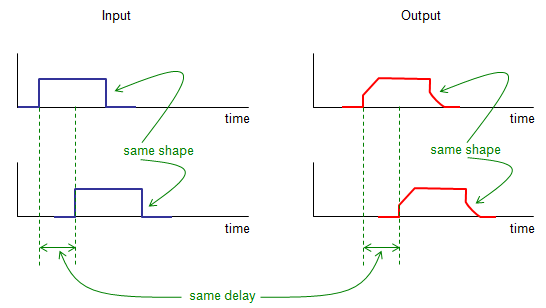
Figure 1. The property drawn as a comparison rather than as a definition. Delaying the input delays the output by the same amount and changes nothing else about it.

• The output is not the same shape as the input : the blue pulse has square edges and the red one is rounded, so this system does something. Time Invarience is about the doing staying the same, not about the output matching the input.
• The two green same shape labels point within a column : the two inputs match each other and the two outputs match each other. Neither label compares the left column with the right.
• The same delay bracket is the whole test : the gap between the two inputs and the gap between the two outputs are drawn as equal. That equality is what the property asserts.
• Only the shift is allowed to change : the lower output is not taller, wider or differently shaped. Any of those would make the system time varient.

Written as a rule rather than a picture, it is one line. If an input x(t) produces an output y(t), then the input x(t - T) has to produce the output y(t - T), for every shift T and every input. The picture above is that line drawn for one pulse and one value of T.

Two things follow from the wording. The shift has to work for every T rather than for a convenient one. It also has to work for every input rather than for the one that was tested. A system that passes for a pulse and fails for a sine wave is not time varient in places, it is simply time varient.

Why the Time Invarience of a system is important ?

The question below is worth asking before the answer arrives, because the cost of losing this property is not obvious. A time varient system still works and still produces output. What it stops doing is allowing anything measured once to be trusted later.

The answer is pretty obvious. Let's suppose you have a system which is Time Varient. You put a certain input and investigated all the characteristics of the input with a lot of time and effort. But you would not be able to reuse the result because when you reuse it, time is different and the result will be different as well. It is like... you have a computer. you would get different result from an exactly same program every time you run it.

The only case you can reuse the result is to make a lot of further efforts to find out the rules to show how the output changes depending on time. Unfortunately you cannot guarantee that you can find the rule. Even though you are lucky enough to find the rule, your model for the system will be extremly complicated.

There is a sharper way to put the same point. A time invarient system can be described once and the description keeps working. A time varient one has to be described again every time it is used, and a description that stops being true is barely a description at all.

What that description usually is makes the value concrete. Send a single impulse into a system and record what comes back, and the recording is the impulse response. For a time invarient system that one recording answers every later question, because the answer to an impulse at any other moment is the same recording shifted.

The signal representation page uses exactly that. It breaks an input into ten shifted impulses, convolves each one with the impulse response, and adds the results. Every one of its ten tracks uses the same impulse response, and only Time Invarience makes that legitimate.

The cost of losing the property is more than accuracy. Without it the system needs a different impulse response for every instant, so the single recording becomes an endless table and convolution stops being one operation. Transforms fail for the same reason, because turning a convolution into a multiplication assumes one response rather than many.

• One measurement, reused forever : that is the whole benefit, and the impulse response is the measurement.
• Shifting the impulse shifts the answer : without that, knowing the response at one instant says nothing about any other instant.
• Convolution depends on it : a single impulse response used at every position is what the operation assumes, and a time varient system breaks the assumption.
• So do the transforms : convolution becomes a multiplication in the z or frequency domain only for a system that does not change.

How to tell whether a system has it

The definition gives a procedure, and it is short enough to run in the head. Delay the input and work out the output. Then work out the output for the undelayed input and delay that instead. The system is time invarient when the two agree for every delay and every input.

The order of the two operations is the entire test. Delaying first and delaying last have to give the same answer, which is why the property is sometimes stated as the system commuting with a delay.

Running that test over the usual textbook systems separates them cleanly. Every row below was checked by generating random inputs, applying the two orders, and comparing the results sample by sample.

• A constant multiplier is safe and a varying one is not : 3 x[n] passes and n x[n] fails, because the second one asks what the index is before deciding what to do.
• Any operation on the time axis itself fails : scaling it, reversing it or sampling it at every second point all make the result depend on where the origin sits.
• Memory is allowed : x[n] - x[n-1] looks at the past and still passes, because it looks at the same relative past wherever it is applied.
• The test is a failure test : one input and one delay that disagree settle the matter, while agreement on a few examples proves nothing.

The last column is the one worth reading carefully, because it shows the two properties are independent of each other. Squaring each sample is time invarient and not linear. Multiplying by the index is linear and not time invarient. A system can have either, both or neither.

That independence is why the two words are always written together. LTI is a pair of separate conditions rather than one idea with two names, and the linearity page takes the same pairing from the other side.

Time invarient over what window ?

Everything above treats the property as something a system either has or does not have. Real systems do not divide that cleanly. A radio channel changes whenever anything in it moves, so it is time varient by nature. The useful question is not whether it changes, but how long it stays still enough.

The rate of change follows from the movement. A terminal moving at speed v shifts the carrier by v times the carrier frequency divided by the speed of light, which is the Doppler frequency. The channel then decorrelates over a time set by that shift. One common definition puts the coherence time at the square root of 9 over 16 pi, divided by the Doppler frequency.

That constant works out at 0.423. Figure 2 draws one such channel at 300 km/h against the windows that matter to a receiver.

Figure 2. One fading channel at 300 km/h and three windows laid against it. Over one symbol the curve barely moves, over a pair it moves a little, and over the coherence time it moves enough to matter. Time Invarience is an assumption with a length.

• The curve is a real calculation : six rays with random phases and angles, added at a Doppler frequency of 556 Hz, which is 300 km/h at 2 GHz.
• The shortest bracket is nearly flat : across one OFDM symbol the channel barely changes, which is why a system may treat it as constant within a symbol.
• The middle bracket is where schemes begin to suffer : a pair of symbols is the window an STBC block needs, and the curve has begun to move across it.
• The longest bracket is where the assumption expires : by the coherence time the gain is visibly different, so anything measured at the start is no longer valid by the end.

The table puts numbers on the same picture across a range of speeds. The last column is the one that decides whether a scheme works, because it says what fraction of the channel's useful lifetime a pair of symbols consumes.

The bottom two rows explain a result from elsewhere on the site. At 300 km/h a pair of symbols spans 18 per cent of the coherence time, and the STBC page measures the resulting leakage at 15 dB below the wanted signal. Those are the same fact stated twice, once as a fraction of a window and once as an interference level.

The same reasoning explains why LTE places its transmit diversity pair across frequency rather than across time. Moving the pair into two adjacent subcarriers replaces the demand for Time Invarience over 133 microseconds with a demand for flatness over 15 kHz, which the SFBC page works through.

The practical form of the property is therefore a deadline rather than a yes or no. Channel estimates are repeated because they expire. Reference signals are sent periodically for the same reason. A system is designed so that everything depending on one measurement finishes before that measurement stops being valid.

• Real channels are time varient and treated as invarient anyway : the approximation is made deliberately and given a lifetime.
• Speed sets the lifetime : 76 ms at walking pace and 761 microseconds at 300 km/h, a factor of a hundred across the range a network has to serve.
• Every scheme that assumes a constant channel has a deadline : channel estimation, transmit diversity and equalisation all measure once and use the result for a bounded time.
• Missing the deadline shows up as interference : the assumption does not fail loudly, it degrades, which is what the 15 dB figure on the STBC page measures.