As you start studying Signal Processing, one of the terminology that you come across the most frequently would be 'Sampling Theory' or 'Nyquist Sampling Rate', 'Over Sampling', 'Under Sampling' etc. I may sound easy, but do you really understanding the practical meaning of those words ? or the importance of them ?

I would not write down the dry definition of those terminologies. If you google it, you would easily find the dictionary type of definition.  In this page, I would take a rather intuitive / practical approach. The story will get very long and it would take long time for me to complete this page.. here goes just the beginning.

• How fast does the sampling have to be ?
• What is the Nyquist Sampling Rate ?
• What happens below the Nyquist rate ?
• Does any rate above 2 fW really work ?
• How do you stop aliasing before it happens ?
• Reference

How fast does the sampling have to be ?

The first step in most Digital Signal Processing would be to sample analog signal and convert it into a digital form. Then the question is how often do we have to sample the original analog signal. Let's assume that we are given an analog signal as (A).  Now we are sampling the original signal (A) with the several different sampling rate as in (B), (C), (D). Then the question is "which (B,C,D) would best represent the original signal (A) ?'. In order words, if we convert the sampled signal (B, C, D) back to analog signal (E, F, G), which of E, F, G would be the closest (most similar) to the original signal (A) ?.

The answer would be simple and intuitive. You would easily pick (C) as the best answer.

Yes, you are right. The best answer is (C). You don't need to try to understand such a boring things like Sampling Theory.

Then what is the problem ? Just sample the signal at as high rate as possible.

It would be OK just to increase the sampling rate if you don't need to think of the cost and any other design limitation.

To sample the signal at high rate, you need high speed ADC and large memory capacity and various high processing power which is not always acceptable.

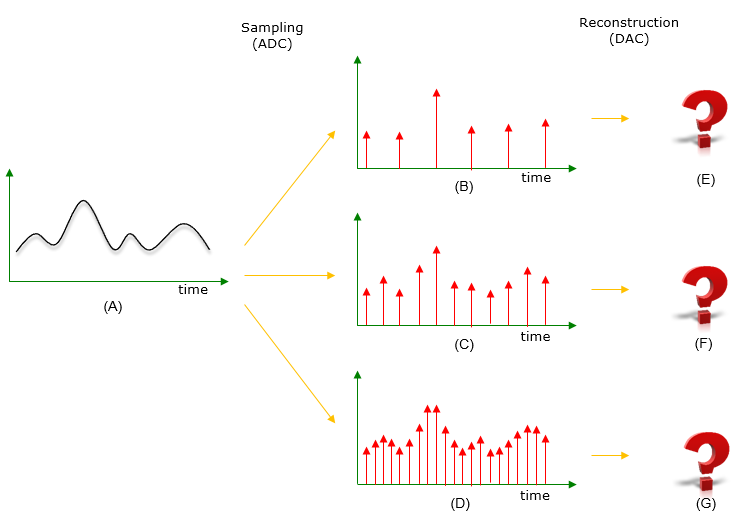
Figure 1. The question drawn, with the answer deliberately withheld. The three reconstructions on the right are question marks rather than waveforms, and that is the point. Nothing tells you what comes back until you know how fast the samples were taken.

• Only the middle column is under your control : the analogue signal on the left and the reconstruction on the right are both given. The sampling rate is the one decision in the picture.
• Each row down the middle takes more samples of the same signal : the stems in (B) are sparse, (C) is denser, and (D) denser again. Nothing else about the three differs.
• The question marks are the honest answer : reconstruction is drawn as unknown because it is unknown until a rule fixes the rate. The next section supplies that rule.

The cost argument above deserves a number, because it decides the answer in practice. Doubling the sampling rate doubles the samples per second, so it doubles the memory a recording needs and doubles the arithmetic every later stage has to perform. The converter itself is the harder part, since a faster converter costs more power and usually gives up resolution to get the speed.

That trade is what makes an obvious question an interesting one. Sampling faster is always safe and never free, so the useful question is not which of the three rows looks best. It is how slowly you can afford to go without losing anything, and that is the question the next section answers.

• Faster sampling is never wrong, only expensive : memory, processing and converter power all scale with the rate, and converter resolution usually falls as the rate rises.
• The interesting number is the minimum, not the maximum : any rate above the threshold works, so the whole of sampling theory is about locating that threshold.

What is the Nyquist Sampling Rate ?

Now let's change a question a little bit as follows : What is the minimum sampling rate that would not lost any critical information of the original signal ?

There is where the Sampling Theory kicks in.

I will just give you the answer first. The minimum sampling rate that meets the requirement is called 'Nyquist Sampling Rate'. You would hear of this term over and over whenever you read any material about sampling theory.

The answer would be as illustrated below. As you see, the answer would take a little bit different form depending on the nature (frequency spectrum) of the original signal.

In case (A), the original signal has only one component with frequency fm. In this case, the Nyquist Sampling Rate is 2 times fm. So any sampling rate which is equal to or greater than twice of fm (2 x fm) would reserve all the critical information contained in the original signal.

In case (B), the original signal is made up of multiple frequency component starting from 0 frequency to fH. In this case, the Nyquist Sampling Rate is 2 times fH. So any sampling rate which is equal to or greater than twice of fH (2 x fH) would reserve all the critical information contained in the original signal.

In case (C), the original signal is made up of multiple frequency component, but starting frequency is not 0. It starts from fL frequency to fH. Let's denote the difference between fH and fL as fW(bandwidth of the signal). In this case, the Nyquist Sampling Rate is 2 times fW (Note that the Nyquist Sampling Rate is not 2 x fH). So any sampling rate which is equal to or greater than twice of fW (2 x fW) would reserve all the critical information contained in the original signal.

Figure 2. Three spectra and three answers. The first two give twice the highest frequency, and the third gives twice the width instead. That third row is worth reading twice, because the rest of this page has to qualify it.

• The left column decides the right column : the rate follows from the shape of the spectrum. Knowing the highest frequency in a signal is not enough on its own. You also need to know the lowest.
• Case (A) and case (B) give the same answer : a single tone at fm and a band reaching up to fH are both measured from zero. Both therefore come out at twice the top edge.
• Case (C) is the surprise : the band starts at fL rather than at zero. The rate drops to twice the width fW rather than twice fH, so a band from 60 to 80 MHz needs 40 MHz rather than 160.
• The figure writes all three with a greater than or equal sign : fs greater than or equal to 2fm, 2fH and 2fW. That sign is exactly right for the first two rows, and the third needs a qualification that appears further down this page.

Two questions usually follow Figure 2, and the second is the one that gets skipped. The first is why the factor is two rather than three or one and a half. The second is whether the sign should really be greater than or equal, or strictly greater than.

The factor of two comes from counting unknowns. A sinusoid at a known frequency carries two numbers, its amplitude and its phase, so recovering it needs two measurements per cycle and no fewer. Two samples per cycle of the highest frequency present is therefore an information bound rather than a rule of thumb.

The sign is stricter than it looks. Sample a sine wave at exactly twice its frequency, and every sample can land on a zero crossing. The recorded signal is then a row of zeros, and the tone has vanished. The safe statement is therefore strictly greater than twice the highest frequency. Real designs leave a margin well beyond that, for the filter discussed at the end of this page.

• Two samples per cycle is a count of unknowns : amplitude and phase are two numbers. Two measurements per cycle is therefore the least that can describe a sinusoid.
• Exactly twice is not enough : a sine sampled at precisely 2fm can be caught at its zero crossings every time and disappear completely. The rate has to exceed the bound rather than meet it.
• The bound is about the spectrum, not the waveform : a violent looking signal can be slow to sample if its spectrum is narrow. A smooth looking one can be expensive if its spectrum is not.

What happens below the Nyquist rate ?

Everything so far has been about staying above a threshold. What that threshold protects against is the subject of this section. It has a name most readers will already have met, and a piece of arithmetic that far fewer have ever written down.

Then, you would have a question : What would happen if we sample the signal at lower rate than Nyquist Sampling Rate ?

This is a very important point of Sampling Theory and it would require pretty long explanation. The simple answer is 'Sampling at lower than Nyquist Rate would cause Aliasing'.

I know this would not make much sense to you if you are completely new to this area. I will post further details of this next time.   

Those further details follow here. The arithmetic behind aliasing fits in one line, and everything else in this section is a consequence of it. Sample a tone at frequency f with a rate fs. The samples you record are identical to those a tone at f minus fs would have produced, and to those from f plus fs, and from any whole number of steps either way.

Take a rate of 100 MHz. A tone at 30 MHz stays at 30. A tone at 70 MHz gives the same samples as one at 70 minus 100, which is minus 30. In a real signal a negative frequency is indistinguishable from its positive twin. Both tones therefore appear at 30 MHz, and Figure 3 draws that.

Figure 3. The one picture that explains the word aliasing. A frequency above half the sampling rate arrives under an assumed name, and the name it takes belongs to a real frequency that may also be present.

• The fold is about fs over 2, not about fs : 70 lands on 30 because both sit 20 MHz from the 50 MHz line. One is above it and one below. Half the sampling rate is the mirror.
• The pattern repeats for ever : 130 MHz also lands at 30, and so does 170, and 230. Every frequency the converter can be shown maps into the range from zero to fs over 2.
• Aliasing is loss, not distortion : the two sets of samples are equal, digit for digit. There is nothing left in the recording that distinguishes them, so no filter or algorithm applied afterwards can separate them.

The practical damage usually arrives from outside the wanted band. An interferer at 130 MHz is far away from a wanted signal at 30 MHz, and a 100 MHz converter drops it directly on top. Distance in frequency is no protection once sampling has happened, which is why the last section of this page is about a filter rather than about arithmetic.

A familiar version of the same effect happens with light rather than with radio. Film a wheel with a camera taking 24 frames a second, and a wheel turning slightly faster than 24 revolutions a second appears to crawl backwards. The camera is a sampler, the rotation rate is the tone, and the backwards crawl is an alias.

• An out of band interferer is the usual cause : the converter folds in anything it can see, whether or not the wanted signal is anywhere near it.
• Amplitude survives the fold : a strong interferer arrives as a strong alias, so a distant but powerful signal can dominate a weak wanted one.

Does any rate above 2 fW really work ?

Case (C) of Figure 2 is the row worth returning to, because it is stated more generously than it can be kept. Twice the width really is the minimum rate. The figure then writes greater than or equal, and the rates above that minimum do not all work.

Take the example from the bullets under Figure 2, a band running from 60 to 80 MHz. The width is 20 MHz, so twice the width is 40. Sampling at 40 works, and sampling at 45 does not. At 45 MHz a tone at 60 lands at 15 and a tone at 75 also lands at 15, by the folding arithmetic of the previous section.

The reason is that folding has to place the whole band between zero and fs over 2. No part of the band may land on any other part. That succeeds only for particular rates, and Figure 4 shows which ones for this band.

Figure 4. The usable rates come in bands rather than as everything above a threshold. For this signal only four regions work. The lowest of them is a single value, because the band edge happens to be a whole multiple of the width.

• The gaps are the finding : 45 and 50 MHz both sit above twice the width and both alias. Being above the minimum is necessary and it is not sufficient.
• The lowest zone is a single value here : 40 MHz works exactly because 80 is four times 20. Move the band to 65 through 85 and the exact minimum stops being reachable at all.
• The widest zone is the safe one : from 160 MHz upward every rate works, because that is ordinary Nyquist on the top edge. Everything below it buys a lower rate by accepting a narrower window of choices.

Choosing a rate from one of those lower zones on purpose is called bandpass sampling, or undersampling. It is what lets a receiver digitise an intermediate frequency far above the converter rate. The RF receive chain page works through a case where an IF around 170 MHz is sampled at 80 Msps. That looks like a violation of Nyquist, and it is not one.

Two warnings belong with that technique. The folded band is reversed in frequency whenever n is even, so the spectrum arrives mirrored and the receiver has to undo it. The sampling clock also has to be far cleaner than the rate alone suggests. Jitter is judged against the input frequency rather than against the sampling rate.

• Twice the width is a floor, not a licence : the condition is 2 fH over n at most fs, and fs at most 2 fL over n minus 1, for some whole number n. A rate outside every such zone aliases.
• Bandpass sampling moves work from the converter to the filter : a slower converter becomes possible. The analogue filter in front of it has to be a good deal sharper.
• Jitter is measured against the input, not the clock rate : sampling a 170 MHz signal at 80 Msps still needs the timing accuracy of a 170 MHz signal.

How do you stop aliasing before it happens ?

Aliasing destroys information at the moment of sampling, so every cure has to act before that moment. The cure is an analogue filter in front of the converter, and its name says what it is for.

The job of an anti-alias filter is narrow and strict. It has to pass the wanted band and reject everything that would fold into it, which for ordinary baseband sampling means everything above half the sampling rate. What it fails to remove, the converter folds inward, and nothing downstream can undo that.

The difficulty is the width of the transition. Sample a signal that reaches 20 MHz at 44 MHz. The filter then has to be flat to 20 and deeply down by 22, which is a steep analogue filter and an expensive one. Sample the same signal at 160 MHz instead, and the filter has from 20 MHz to 80 MHz to do the same job. A gentle filter then suffices.

That trade is the practical argument for oversampling. Running the converter faster than the theory demands buys a cheaper analogue filter. The extra samples are then removed digitally, where a steep filter costs arithmetic rather than components. Converters designed around this idea are common, and the sampling theorem is what sets the floor they oversample against.

Bandpass sampling changes the filter rather than removing the need for one. The filter in front of the converter becomes a bandpass filter. It must reject everything outside the wanted band on both sides, not merely above half the sampling rate. A signal that folds in from below is exactly as damaging as one that folds in from above.

• The filter has to be analogue and it has to be first : once the samples exist the aliased energy is part of them. A digital filter arrives too late to help.
• Oversampling buys filter margin : the gap between the top of the wanted band and half the sampling rate is the room the filter has to work in. Widening that gap is usually cheaper than sharpening the filter.
• Decimate afterwards, in the digital domain : the extra rate is only needed at the converter. A digital filter then removes what the analogue one could not, and the rate drops back.
• A bandpass design needs rejection on both sides : energy below the band folds in just as readily as energy above it, which is what makes undersampling demanding rather than free.

Reference

[1] SIMULATION OF DIGITAL COMMUNICATION SYSTEMS USING MATLAB By Mathuranathan Viswanathan

[2] USING MATLAB TO ILLUSTRATE THE' PHENOMENON OF ALIASING' by Sol Neeman, Johnson and Wales University

[3] EE 424 #1: Sampling and Reconstruction