Intuitive understanding of Fading would be simple, but the detailed description is pretty difficult and would be even more difficult to understand the details without going through the complicated mathematical process. This page would start with Intuitive description and try to keep adding the details one by one. It will take long time to complete the pages and will split this into multiple pages if it goes too long.
Followings are the topics in this page.
- Intuitive Understanding
- Major Components of Fading
- Fast Fading and Slow Fading
- Path Loss and Shadowing
- Channels with MultiPath
- Interpretation of Fading Channel Profile
- Correlation among Channels
- How these correlation are derived ?
- How to derive MIMO coeifficient matrix mathematically from Diversity coefficient matrix ?
- Going Back to 3GPP Correlation Tables
- Doppler Spread
- High Speed Training Model/Scenario
- General Concept of Fading Channel Simulation
- Fading Channel Model Examples
- Get the Test Procedure and Log / Amarisoft TechAcademy
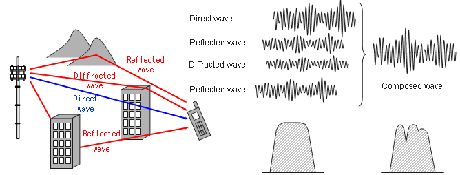
In most of the wireless communication environement, a signal out of a transmitter radiate into wide direction and these radiated signal takes different path and arriving at the reciever at different timing and with different signal strength(amplitude). As a result, the signal coming into the reciever is the composite of all the components. As you may learned in high school physics, when thetwo copies of the signal get combined the resulting signal can be an augmented signal or attenuated signal depending on whether the two signal constructively combined or destructively combined.
Then what determines whether the signals constructively combine or destructively combine ? The answer also come from high school physics. The phase of the two signal determines whether the signal constructively combine or destructively combine.
In wireless communication environment, many copies of the signals get combined at the reciever side and some of them constructively combines and some of them destructively combines. So final result of combination of all the incoming signals become very complicated and the combined signal becomes drastically different from the original signal tranmitted from the source. In most case, the quality of the combined signal at the reciever gets poorer (deteriorated) than the original signal. This kind of process of signal deterioration by the multiple propogation path of a signal is called 'Fading'. When we say "Fading", it usually implies "Signal quality gets bad".
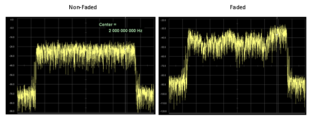
For more intuitive unerstanding of the fading, I will show you a couple of different aspect of fading you can mesure using various equipments.
First, let's compare a faded signal and non-faded signal using a spectrum analyzer. You would get the two results as follows and you will see the highly fluctuating amplitude across the channel bandwidth. (Note : These two capture are not the one from the same signal, so comparing the absolute value of the amplitude does not make any sense. Just take the image of overall amplitude profile).
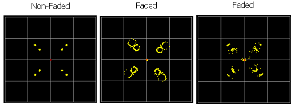
Now let's look at how the fading influence the signal quality decoded by the reciever. Look at the following samples of constellation for faded and non-faded signal.
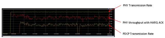
Now let's get into even further and I think this is the thing that you would be most interested in. How this fading would influence the final performance. Following graph shows the data rate at PHY layer and PDCP layer. The plot showing at the top (labeled as 'PHY Transmission Rate') is the amount of data being transmitted per second by PHY layer of the transmitter. The plot in the middle (labeled as 'PHY throughput with HARQ ACK' is the amount of data getting ACKED per second from the reiever PHY layer. You see there is pretty much gap between the two plots. It means that a considerable portions of the data were failed to get properly decoded by the reciever and the reciever sent NACK for the data. Normally in this case, the transmitter PHY layer retransmits the previous data rather than moving into the next step of the transmission.
The plot at the bottom (labelled as 'PDCP Transmission Rate') is the amount of data being sent to the lower layer from the transmitter's PDCP layer. You will see another gap here. It is not easy to explain exactly what is causing this gap. In this case, some portions of the gap would come from the overhead of higher layer data structure but majority of the gap would be because PDCP cannot push the data down to the lower layer since PHY layer is too busy with retransmitting the previous data rather than transmitting the new data coming from the higher layer.
There are many factors generating Fading effect. Followings are the list of components (factors) of fading we can think of.
- Path Loss
- Fluctuation of the received signal power
- Fluctuations in signal phase
- Variations of Angle of arrival of received signal
- Reflection and diffractions from various object
- Recieved power variation created by multi path
- Frequency Shift(Doppler shift)
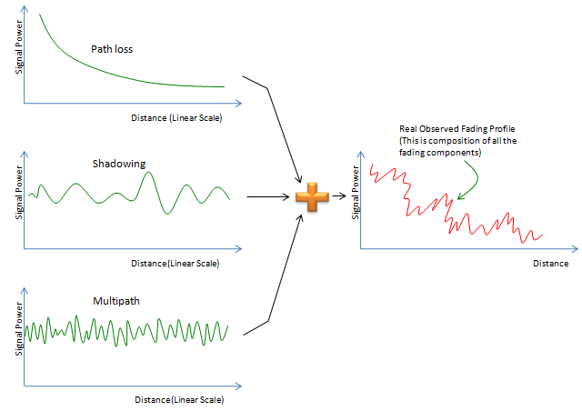
To study on fading requires the detailed understanding of each of these components. If I express some major components in visual form, it can be presented as follows. Just from the high level view, you should see some typtical pattern from this representation. First notice that the horizontal axis represents 'Distance in Linear Scale'. You may have seen a lot of different plots in various textbook and get confused by those. One of the first step to remove those confusion would be clearly understanding the meaning of axis of the graph. Even for the same things, you would see different shape of plots if you define the meaning of the axis differently. One of the factors from various text confusing you the most is the scale of each axis. For example, in case of path loss graph in some textbook where they represent the axis in log scale you would see a straight line, but in this page you are seeing a kind of negative exponential graph since the axis is represented in linear scale.
Now let's look into each of the graphs.
Path loss is just gradually decreases but not much of fluctuation. In the second plot, you see some fluctuation of the signal strength but the fluctuation frequency over the distance is not that high. In the third plot, you see fluctuations of signal strength and the fluctuation frequency is also pretty high.
When you observe a real received signal, you wouldn't see these factors in separate form as in the graph on the left side. What you see at the real reciever is the result of summation of all the factors and it is like the graph on the right side.
Probably the words you might have heard the most frequently when you talking about fading would be 'Fast Fading', 'Slow Fading'. Intuitively it sounds simple. But not easy to find clear/technical defintion for these. How fast it should be to be Fast Fading ? How slow it should be to be Slow Fading ?
I found a very good definition and technical explanation from the reference [2]. It states as follows:
Fast Fading is used to describe channels in which Channel Coherence Time < Tansmission Symbol Time. Fast Fading describes a condition where the time duration in which the channel behaves in a correlated mannel is short compared to the time duration of a symbol. Therefore, it can be expected that the fading characteristic of the channel will change several times while a symbol is propagating, leading to distortion of the baseband pulse shape. Analogous to the distortion described as ISI, the distortion take place because the recieved signal's components are not all highly correlated throughout time. Hence, fast fading can cause the baseband pulse to be distorted, resulting in a loss of SNR that often yields an irreducible error rate. Such distorted pulses cause synchronization problems (failure of phase-locked-loop recievers), in addition to difficulties in adequately defining a matched filter.
Slow Fading is used to describe channels in which Channel Coherence Time > Tansmission Symbol Time. Here, the time duration that the channel behaves in a correlated manner is long compared to the time duration of a transmission symbol. Thus, one can expect the channel state to virtually remain unchanged during the time in which a symbol is transmitted. The propaging symbols will likely not suffer from the pulse distortion. The primary degradation in a slow-fading channel, as with flat fading, is loss in SNR.
Path Loss and Shadowing may not be considered to be a part of Fading in narrow sense, but it can be considered as a factor causing the fading in wider sense. Understanding or Modeling the path loss is not that difficult. You may see a mathematical model which you were faimilar with in your high school math. The famous format of anti-proportional to 'something squared'.
Modling for Path Loss is done with the respect to the distance between a transmitter and receiver. The key question is ..
Test A) When a transmitter antenna is transmitting a certain (fixed) amount of energy and you put a measurement antenna which is a certain distance (let's call this distance as 'd') and measure the received(measured) energy. Once you get the value at a certain 'd', write down the value. And then move the reciever antenna a little bit further and do the same measurement and write down the value. Repeat this process as you move 'd' further and further and collect all the measured value and plot it on the graph with horizontal axis = d and vertical axis = measured energy level (power). How would the plot look like ? Can you come up with an equation to represent the graph ?
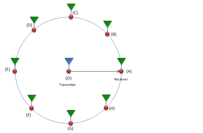
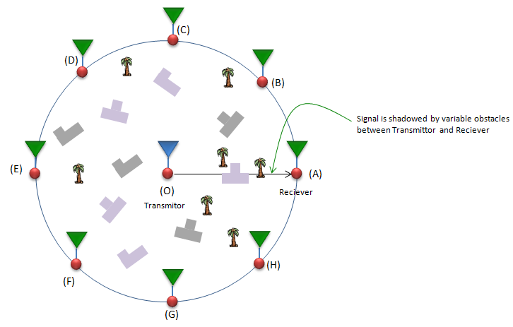
Test B) Now let's try a little bit different type of measurement. This time, draw a circle with radius d with the transmitter antenna at the center. and then put several antenna along the circumference and measure the received power at each antenna and plot the value with horizontal axis = location of receiver antenna and vertical axis = measured energy level (power). How would the plot look like ?
Test C) Now let's think about two test environment. In one setup there is no obstacles between the reciever and transmitter antenna (Let's call this as 'Setup A'). In the other setup, there are a lot of obstacles (like building, tree, houses, mountain etc) between the transmitter antenna and reciever antenna (Let's call this as 'Setup B'). Then you do the measurement described in Test B) for both setup and compare the result. Would you see any difference ? what kind of difference would you see ?
These three test will be used as a basis for modeling following cases. (Details will come later)
< Path Loss Model in Free Space >
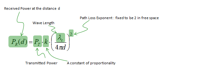
The first thing we can think of is a kind of ideal case called 'Free Space'. In this case, we assume that there is no obstacles between the transmitter and reciever antenna.
In this case, the measured power at every reciever antenna at the same distance from the transmitter antenna would be same and the received signal power can be modeled as follows. (Basically this equation is a form of Frris' Transmission Equation )
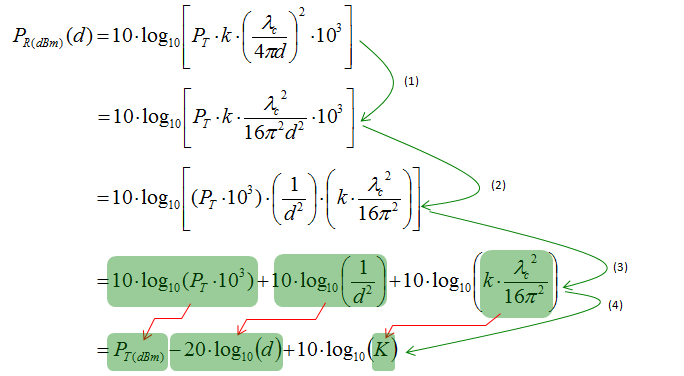
If you want to convert this equation to a form which most of RF engineers are more familiar with (dBm scale), you can just apply 10 log( ) on both side and go through following steps. Of course, you don't have to memorize the each of these steps. Just try to understand overall concept and logic of this process.
< Path Loss Model in Real Situation : Shadowing >
Life would be much easier if the condition between the transmission antenna and reciever antenna is always as decribed in previous case (Free Space).
In real life situation, it is highly likely that you would see a lot of obstacles (like building, Tree, mountain etc). If I draw this situation in a little bit simplified way, it would be as follows.
The path loss at a certain distance can be expressed as follows. Compare this with the free space case. What kind of difference do you see ?
In case of free space model, once the distance is determined the received power can be determined automatically meaning that if d is fixed(same), you would get the same measured value (recieved power) for every measurement. But in this case, you cannot gurantee the same measured value even though the distance is same. Even though d is same, you would get the different measured value if beta (Path Loss Exponent) is different or epsilon (Random Variable) is different.

Then the question would be 'How the Path Loss Exponent and Random Variable is determined ?'. There is no strict theory that can determine these values deterministically. It is usually determined empirically. According to various researches,
- Path Loss Exponent depends on the frequency, antenna height and propagation environment.
- In case of free space, it is 2
- it can be lower than 2 if there is very strong guided wave phenomena (as in urban street)
- n become larger when there is
- Random Variable epsilon turned out to be Zero-mean Gaussian
If you apply Log (10 log[ ] more specifically) to both side, you can get a linear equation in dB (dBm) scalse as shown below.
![]()
A defining characteristic of the mobile wireless channel is to build up a mathematical model for the variations of the channel strength over time and over frequency. There are mainly two factors influencing the variations of the channel strength as listed below.
- Large-scale fading : This can be called as 'Slow fading' as well and this is mainly caused by path loss of signal as a function of distance and shadowing by large objects such as buildings and hills. This occurs as the mobile moves through a distance of the order of the cell size, and is typically frequency independent.
- Small-scale fading : This can be called as 'Fast fading' and this is mainly caused by the constructive and destructive interference of the multiple signal paths between the transmitter and receiver. This occurs at the spatial scale of the order of the carrier wavelength, and is frequency dependent.
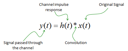
As a starting point, please... please ... please ... read very carefully about the section of Signal Presentation, Impulse Response and Convolution section before you go deeper into this section.
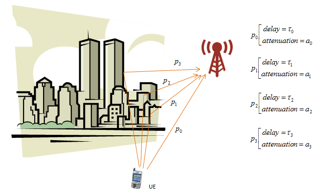
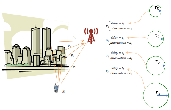
Let's suppose we have a case as shown below. A UE is communicating with a eNodeB and there is a lot of building between the UE and the eNodeB. You may intuitively guess the eNodeB would get the multiple copies of the same signal from UE because the same signal can reach the eNodeB via multiple path as shown below. Let's assume that we have four different path as shown below. There are two major characteristics of the paths. One is attenuation and the other one is time delay. Of course there would be several additional factors, but these two components would be the largest factors. Let's assume that each of the path has the delay and attenuation as shown below.
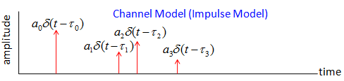
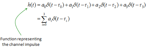
How do we represent a channel using these delay and attenuator factor ? There can be a couple of different ways to represent it, but one of the most common way would be to represent it as an impulse response model. Even though you may not familiar with the term 'impulse response', you may have seen this kind of description if you have any experience of using channel simulators (fader) and dealt with fading profile. Following is the graphical representation of impulse response of the four paths in this example and physical meaning of it. I hope this make sense to you.
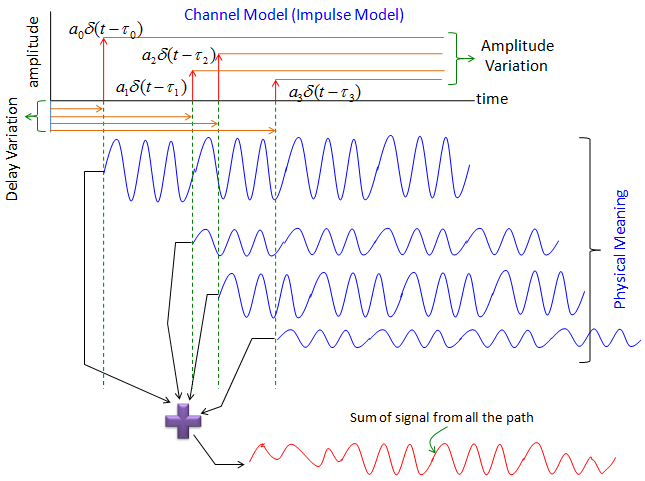
If you represent this impulse response into a mathematical form, it become as follows. If you are not familiar with this kind of mathematical representation. Read again the section of Signal Representation. (When you are first learning this way of signal representation.. you may think .. what the hell is delta function ? Why we need this kind of function ? etc... this is one example why you need to learn those textbook concept).
Let's look into a example that (hopefully) would give you more concrete understanding of these concepts.
Let's suppose that a signal goes through six different path (multipath) as indicated in plot (1). Horizontal axis represents the time delay from the transmission to arrival at the reciever antenna. Vertical axis indicates the amplitude of the received signal. plot(2)~(7) shows the signal going through each path reaching to Rx antenna. If you look at each plots, you would notice that the phase (time delay) and amplitude are different from each other. plot (8) shows the summation of all the plots from (2) through (6). This is the signal being sensed by the recieving antenna.
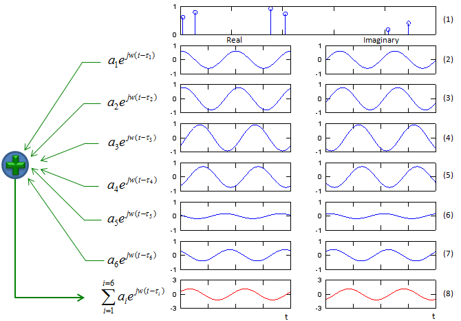
What do you observe from the plot (8) (the sum of all the multipath signal) ? You would notice that the amplitude and phase gets different from the transmitted signal, but overall shape of the signal is same as the transmitted signal. It means that no distortion happened by this multipath.
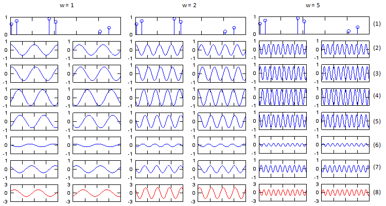
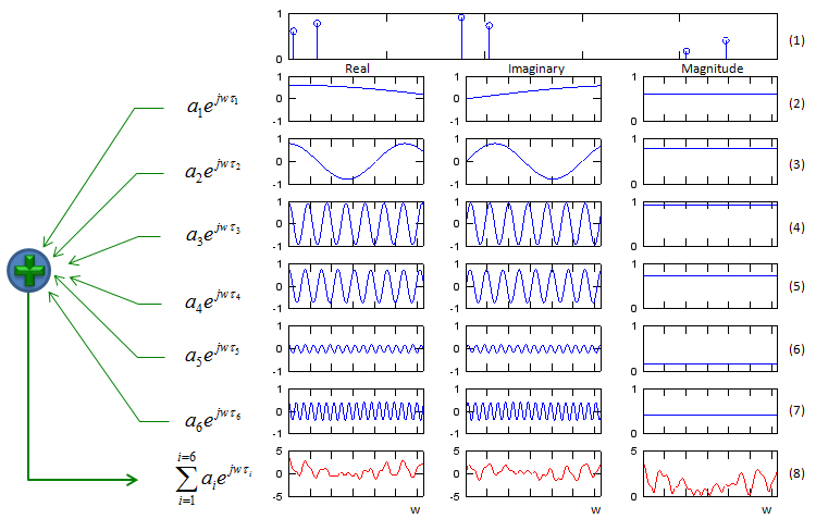
Now let's think of how the received signal is influenced by the multipath with the frequency of the transmitted signal. I created plots for three different frequency (In this case, the amplitude of transmitted signal are same for all frequencies). As you see at plot (8) of each case (w=1,2,5), the amplitude of the total received signal gets different depending on frequency.
Note : This shows the cases of only three different frequencies. Isn't there any way of showing the amplitude of total received signal for all the different frequencies in easier way ? We will look into this shortly.
Following is the Octave source code (I think this would work with Matlab as well) for the graphs shown above, try playing the list 'a' and 'tau', get some intuitive understanding on your own.
a=[0.6154 0.7919 0.9218 0.7382 0.1763 0.4057];
tau=[0.0099 0.0579 0.3529 0.4103 0.8132 0.8936];
t = 0:1/100:2;
w = 5;
N_path = length(tau);
exp_iwt_sum = zeros(1,length(t));
subplot(N_path + 2,2,[1 2]);
stem(tau,a);set(gca,'ytick',[0 1]);set(gca,'xticklabel',[]);
for d=1:1:N_path
exp_iwt = a(d) .* exp(j .* 2 .* pi .* w .* (t .- tau(d)) );
exp_iwt_sum += exp_iwt;
subplot(N_path + 2,2,2*d+1);
plot(t,real(exp_iwt)); xlim([0 2]);ylim([-1 1]); set(gca,'xticklabel',[]); set(gca,'ytick',[-1 0 1]);
subplot(N_path + 2,2,2*d+2);
plot(t,imag(exp_iwt)); xlim([0 2]);ylim([-1 1]); set(gca,'xticklabel',[]); set(gca,'ytick',[-1 0 1]);
end
d = N_path + 1;
subplot(N_path + 2,2,2*d+1);
plot(t,real(exp_iwt_sum),'r-'); xlim([0 2]);ylim([-3 3]); set(gca,'xticklabel',[]); set(gca,'ytick',[-3 0 3]);
subplot(N_path + 2,2,2*d+2);
plot(t,imag(exp_iwt_sum),'r-'); xlim([0 2]);ylim([-3 3]); set(gca,'xticklabel',[]); set(gca,'ytick',[-3 0 3]);
a=[0.6154 0.7919 0.9218 0.7382 0.1763 0.4057];
tau=[0.0099 0.0579 0.3529 0.4103 0.8132 0.8936];
w = 0:pi/100:40*pi;
wmax = max(w);
N_path = length(tau);
Hw_sum = zeros(1,length(w));
subplot(N_path + 2,3,[1 3]);
stem(tau,a);set(gca,'ytick',[0 1]);set(gca,'xticklabel',[]);
for d=1:1:N_path
Hw = a(d) .* exp(j * w * tau(d) );
Hw_sum += Hw;
subplot(N_path + 2,3,3*d+1);
plot(w,real(Hw)); xlim([0 wmax]);ylim([-1 1]); set(gca,'xticklabel',[]); set(gca,'ytick',[-1 0 1]);
subplot(N_path + 2,3,3*d+2);
plot(w,imag(Hw)); xlim([0 wmax]);ylim([-1 1]); set(gca,'xticklabel',[]); set(gca,'ytick',[-1 0 1]);
subplot(N_path + 2,3,3*d+3);
plot(w,abs(Hw)); xlim([0 wmax]);ylim([0 1]); set(gca,'xticklabel',[]); set(gca,'ytick',[0 1]);
end
d = N_path + 1;
subplot(N_path + 2,3,3*d+1);
plot(w,real(Hw_sum),'r-'); xlim([0 wmax]);ylim([-5 5]); set(gca,'xticklabel',[]); set(gca,'ytick',[-5 0 5]);
subplot(N_path + 2,3,3*d+2);
plot(w,imag(Hw_sum),'r-'); xlim([0 wmax]);ylim([-5 5]); set(gca,'xticklabel',[]); set(gca,'ytick',[-5 0 5]);
subplot(N_path + 2,3,3*d+3);
plot(w,abs(Hw_sum),'r-'); xlim([0 wmax]);ylim([0 5]); set(gca,'xticklabel',[]); set(gca,'ytick',[0 5]);
Now we have a channel described in the form of impulse response. Let's suppose that we have a signal x(t) going through the channel. The x(t) will split into multiple pathes in the channel and take the different route and finally recombine at the receiver antenna. What would the signal at the receiving antenna look like ? There is an excellent mathematical tool to give you the answer to this question. It is a tool called 'Convolution'. If you just take the convolution of channel impulse response and input signal (x(t)), you would take the signal at the receiving antenna.
Interpretation of Fading Channel Profile
There are many different ways of modeling the fading channel, but I think the most commonly used model (at least for studying purpose) would be the Rayleigh channel model using Jake's Algorithm (I would say Simplified Jake's algorithm in this note).
Single Path Fading/Jake's Model
I think Single Path Fading based on Jake's model would be one of the most commonly introduced in various textbook or articles mainly for simplicity. The basic concept of the model can be illustrated as below.
NOTE : You may think it odd that I used the term 'single path' here, where the reciever gets the signal from many different directions. Yes, in micro scale you can say this is a multipath model. But when I say 'Single Path' in the title, it is based on a kind of micro model. Each of the arror (signal) in the illustration has a little bit different frequency (due to Doppler shift) and a little bit different phase (due to random phase shift), but overall delay from the receiver (the distance from the reciever to each of the scatterer, that is the radius of the circle, are same). When I say 'Single Path' in this context, it means the overall distance/delay from the scatterer to the reciever.
In practical situation, it is highly likely that the reciever goes through a multipath fading channel. However, in terms of understanding the model, the single path model as shown below would be a good starting point.
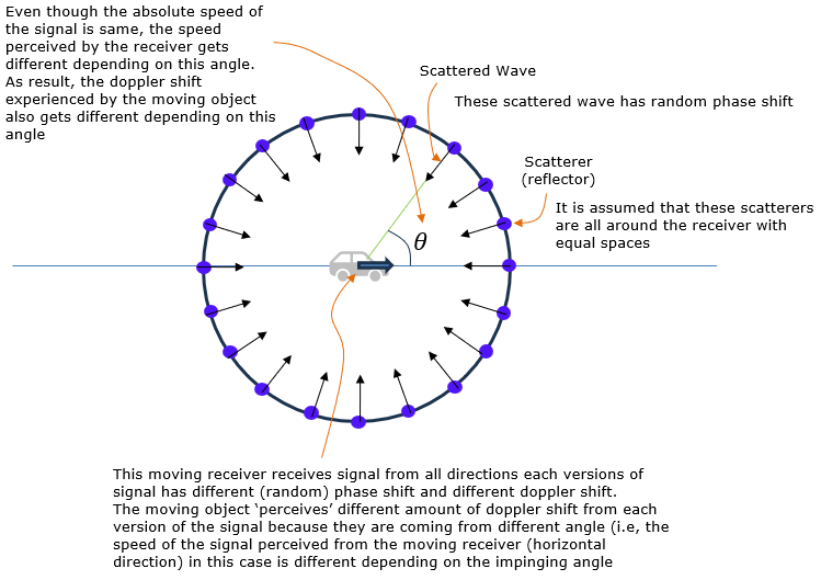
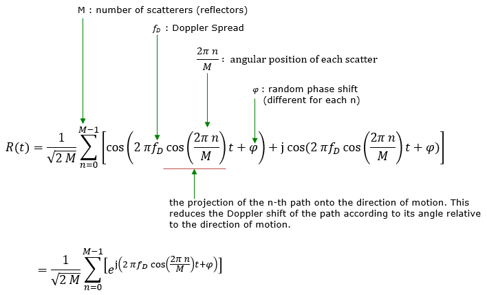
The methematical representation of Jake's model for the illustration above is as follow. R(t) is the total fading by all of the scatterers at specific time (t).
Math itself is not so complicated, but it would take some time (long time) for you to develop an intuition about this equation. At least for me, it took so long time.
NOTE : A tricky part of understanding this equation intuitively would be about doppler part which is represented by fD * cos(2 pi n/M). For this, you may need some additional explanation in detail. Check out Doppler Spread section for additional details.
There are several assumptions for Jake's model. These assumption may be considered as a limitation of this model, but we get such a simple mathematical representation shown above thanks to these assumptions. The assumptions with Jake's model can be summarized as follows.
- Isotropic scattering: This model assumes that the radio waves are scattered equally in all directions. This means that the scatterers around the mobile station are uniformly distributed in all directions.
- Large number of scatterers: The model assumes that there are a large number of scatterers contributing to the multipath components. This allows the model to use the central limit theorem to approximate the sum of all these components as a Gaussian process.
- Random phases: The model assumes that the phases of the signals arriving from different paths are random and uniformly distributed between 0 and 2π. This corresponds to the assumption that the scatterers are located at random positions.
- Flat fading: The model is a model of flat (or frequency non-selective) fading. This means that the model assumes that the bandwidth of the signal is smaller than the coherence bandwidth of the channel. In other words, all frequency components of the signal experience the same amount of fading.
- Stationarity and ergodicity: The model assumes that the statistical properties of the fading process are constant over time (stationarity) and that the time averages and ensemble averages are the same (ergodicity). This allows the model to generate a single realization of the fading process that is representative of its statistical properties.
- Doppler spectrum: The model assumes a certain shape for the Doppler spectrum, which describes the distribution of the Doppler shifts of the multipath components. Specifically, the model assumes a so-called "Jakes' spectrum", which is a bell-shaped curve centered at zero Doppler shift.
|
Fading_Jakes.py |
|
import numpy as np import matplotlib.pyplot as plt import matplotlib.gridspec as gridspec
class JakesGen: def __init__(self, blockSize, fDts, Ns, randomSeed): self.blockSize = blockSize self.fDts = fDts self.Ns = Ns self.state = np.random.RandomState(randomSeed)
def generate(self): # Initialize output y = np.zeros((self.blockSize,), dtype=complex)
# Generate independent in-phase and quadrature components for i in range(self.Ns): # Uniformly distributed angles alpha = (2*np.pi/self.Ns)*i
# Doppler frequency for this component fn = self.fDts * np.cos(alpha)
# Random initial phase phi = 2 * np.pi * self.state.rand()
# Generate in-phase and quadrature components I = np.cos(2*np.pi*fn*np.arange(self.blockSize) + phi) Q = np.sin(2*np.pi*fn*np.arange(self.blockSize) + phi)
# Accumulate components y += I + 1j*Q
# Normalize output y /= np.sqrt(2*self.Ns)
return y
def apply_fading_to_iq_data(iq_data, h): return iq_data * h
# Test the function SampleRate = 30.72e6 N = 10 * np.int16(SampleRate/1000) # Number of samples Ts = 1/SampleRate # Sampling period (1 ms). Timelapse between the two consecutive samples
# Generate 4-QAM IQ data M = 4 # QAM order m = int(np.sqrt(M))
# Generate QAM symbols symbols = [(2*i - m + 1) + 1j*(2*j - m + 1) for i in range(m) for j in range(m)] symbols = np.array(symbols, dtype=complex)
# Repeat symbols to create IQ data iq_data = np.tile(symbols, N//M + 1)
# Ensure iq_data length is N iq_data = iq_data[:N]
# Create JakesGen object. Try out various different values for the following values. Play first with Ns and speed.
randomSeed = None # Random seed Ns = 20 # Number of scatterers
speed = 50 # km/hour v = speed * 1000 / 3600 # velocity in m/s fc = 2000 * 10e6 # frequency in Hz c = 3e8 # light of speed in m/s fD = v * fc / c fDts = fD * Ts # Normalized Doppler frequency blockSize = N # Block size print("fDts = ", fDts) jakesGen = JakesGen(blockSize, fDts, Ns, randomSeed)
# Generate Jake's model h = jakesGen.generate() faded_iq_data = apply_fading_to_iq_data(iq_data, h)
# Create a grid for the subplots gs = gridspec.GridSpec(3, 2)
plt.rcParams.update({'font.size': 7})
# Plot the original and faded data in separate subplots fig = plt.figure(figsize=(6, 8))
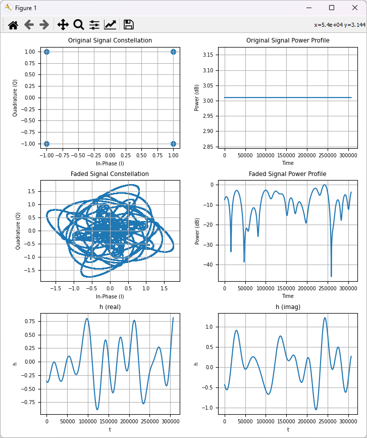
# Original signal constellation ax0 = plt.subplot(gs[0, 0]) ax0.scatter(iq_data.real, iq_data.imag) ax0.set_title('Original Signal Constellation' ) ax0.set_xlabel('In-Phase (I)') ax0.set_ylabel('Quadrature (Q)') ax0.grid(True)
# Original signal power profile ax1 = plt.subplot(gs[0, 1]) ax1.plot(10*np.log10(np.abs(iq_data)**2)) ax1.set_title('Original Signal Power Profile') ax1.set_xlabel('Time') ax1.set_ylabel('Power (dB)') ax1.grid(True)
# Faded signal constellation ax2 = plt.subplot(gs[1, 0]) ax2.scatter(faded_iq_data.real, faded_iq_data.imag, s=1) ax2.set_title('Faded Signal Constellation') ax2.set_xlabel('In-Phase (I)') ax2.set_ylabel('Quadrature (Q)') ax2.grid(True)
# Faded signal power profile ax3 = plt.subplot(gs[1, 1]) power_faded_db = 10*np.log10(np.abs(faded_iq_data)**2) power_faded_db_normalized = power_faded_db - np.max(power_faded_db) ax3.plot(power_faded_db_normalized) ax3.set_title('Faded Signal Power Profile') ax3.set_xlabel('Time') ax3.set_ylabel('Power (dB)') ax3.grid(True)
# Fading process ax4 = plt.subplot(gs[2, 0]) ax4.plot(h.real) ax4.set_title('h (real)') ax4.set_xlabel('t') ax4.set_ylabel('h') ax4.grid(True)
ax5 = plt.subplot(gs[2, 1]) ax5.plot(h.imag) ax5.set_title('h (imag)') ax5.set_xlabel('t') ax5.set_ylabel('h') ax5.grid(True)
fig.tight_layout() plt.show() |
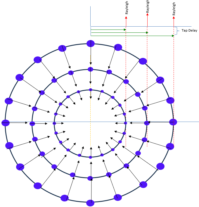
In case of multi path model illustrated as on the left of the following figure, the fading model for each path can be represented as a green circle indicated on the right. Each of the green circle is can be modeled as a single path model as explained above. Each of the circle has different diameter, meaning different overall delay. The total fading that the reciever experience is the summation of all of the green circles.
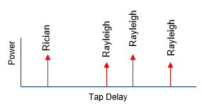
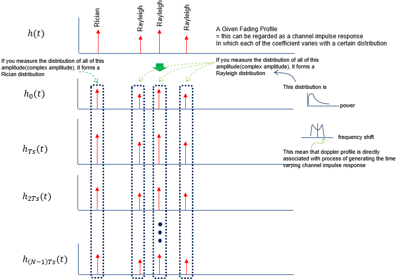
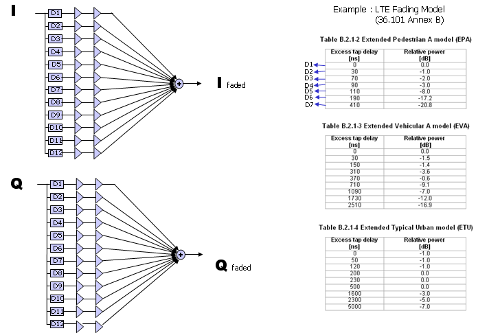
When we specify a Fading Channel profile, we are usually given a table with tap delay and relative power for each tap. You may visualize the table as shown below. Usually those profile table in the specification does not specify statistical information for the tap, but usually some specific statistical profile is associated with each tap. In case of LTE channel profile (Tap Delay Line : TDL), usually each tap is associated with statistical power profile as shown below. Usually the first tap indicates the fading on line of sight path that is modeled in Rician distribution and the remaining taps indicates the fading channel on non line of sight path that is modeled in Rayleigh distribution.
When it comes to using this channel profile in fading implementation. This kind of Tap delay plot can be associated with multiple single channel fading model as illustrated below.
Sound simple ? Yes simple conceptually, but there is a difficulties in reality. It is about how to apply the statistical property associated with each tap.
Each tap is associated with a specific statistical power and doppler profile(i.e, the statiscial power and doppler profile generated by each single channel model explained in previous section).
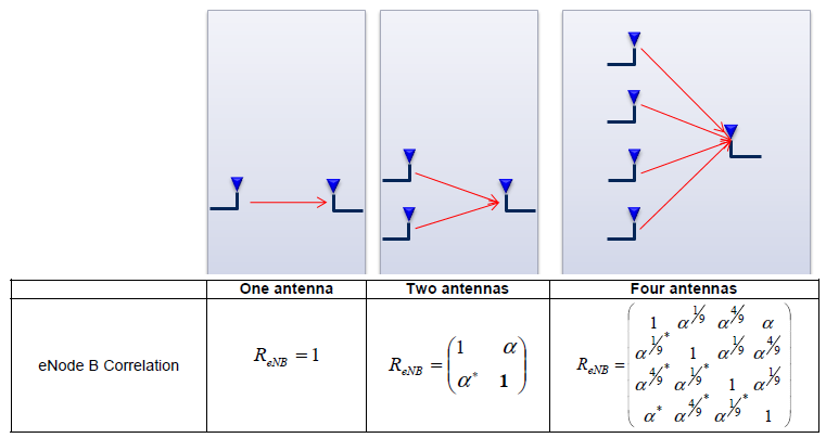
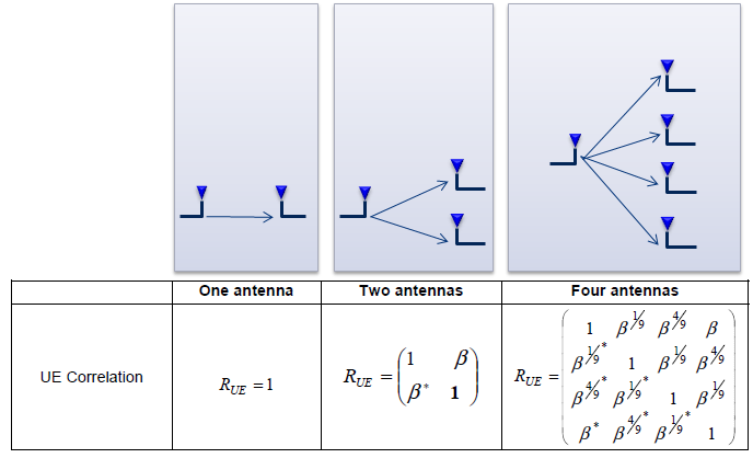
In addition to this delay, gain, PDF, we have to think about the correlations among all the antenna on transmitter and reciever side as follows.
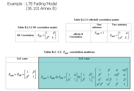
These correlation is defined in 3GPP as shown below and this correlation matrix should be applied to the Fading model when we use multiple antenna configuration.
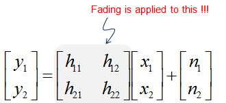
Do you see any difference between the matrix shown above (channel matrix) for 2 x 2 MIMO and the correlation matrix as shown below for 2 x 2 case ?
One obvious difference is size of the matrix. The channel matrix shown above is 2x2 matrix and the correlation matrix for 2 x 2 case shown below is 4x4.
Any idea on how the 2x2 matrix show above is converted to 4 x 4 matrix shown below ?
This is a major topic for following section.
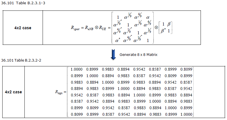
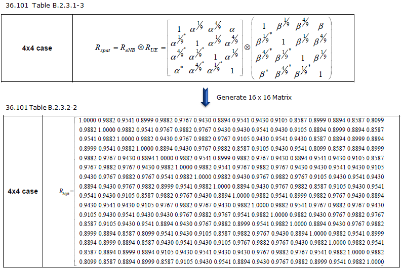
(The full correlation matrices is obtained by Tensor Product/Kronecker product of two antenna correlation matrix)
How these correlation are derived ?
Let's start with the simplest case and add piece by piece until we reach more realistic (complex) cases.
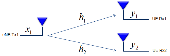
Let's suppose that you have two Tx antenna and one Rx antenna. If draw this situation as in channel model, you can draw this setup as follows. (Let's call this a Case A)
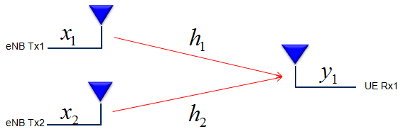
In this setup, you have two channel path(channel coefficient) h1 and h2. Now let's think about all the possible relation between these two channel. If you draw all the possible relationships as a diagram, you may represent as follows.
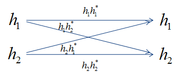
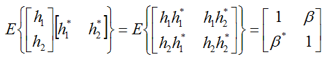
If you represent these relationship between the two channel path (channel coefficient) in a matrix format, you can represent it as follows. (I would not explain it in detail but you would need to have some intuitive understanding of vector/matrix. This is why you should have taken such a boring linear algebra course in the university. If you are really new to this vector/matrix concept, Vector/Matrix page on this site). Be careful, you may get confused with 2 x 2 matrix to be used to model 2 x 2 MIMO channel. (At least I was confused a lot at the beginning. I would not talk too much about it, but I strongly recommend you to compare the two matrix and clearly understand the difference between them). Just to give you the conclusion about the difference between the two matrix, the matrix shown here represents the correlation between each channel path(the path the signal flow through) and the matrix shown in channel model represents the correlation between Tx and Rx antenna.
The 'Beta' value represents the cross correlation between channel coefficient h1 and h2.
Now we have a different case. In this case, you have two Tx antenna and one Rx antenna. If draw this situation as in channel model, you can draw this setup as follows. (Let's call this a Case B)
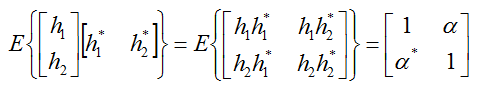
If you represent these relationship between the two channel path (channel coefficient) in a diagram, you can represent it as follows.
If you represent these relationship between the two channel path (channel coefficient) in a matrix format,, you can represent it as follows.The 'Alpha' value represents the cross correlation between channel coefficient h1 and h2.
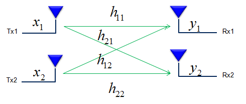
Now let's look into more complicated case. In this case, you have two transmitter antenna and two reciever antenna. The antenna and channel path can be illustrated as follows. You can think of this as a combination of Case A and Case B described above.
Now if you represents the correlations between each of these channel coefficients, it can be represented as follows.
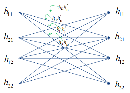
As you did in case A and B, if you represents these correlations in vector/matrix format, you would get a big matrix as follows. How did you get the last matrix ?. Actually it came from the matrix for Case A and B described above. If you clearly understood the meaning of Beta and Alpha in Case A and B, you would easily understand how each of the elements in this big matrix can be represented as 'Alpha' or 'Beta'.
Then what about the '?' part ?
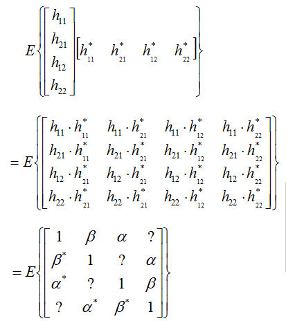
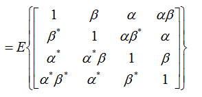
what about the '?' part shown above ? Filling out these '?' is not so straigtforward. If you brow the statical concept (I cannot explain though :)), those parts are the places where the correlation between part of Case A and part of Case B and can be filled as follows.
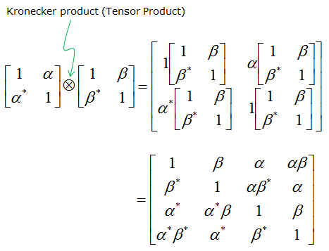
How to derive MIMO coeifficient matrix mathematically from Diversity coefficient matrix ?
I have explained how we got 2x2 MIMO correlation matrix from physical perspective and the each elements of 2 x 2 MIMO matrix can be derived from the elements of 2x1 Diversity matrix. I strongly recommend you to try to get familiar with this concept and build your own intuition. But as the number of antenna increases, deriving all the correlation matrix as I described above would not be that easy. Fortunately there is a mathematical way of deriving the MIMO correlation matrix from Diversity Correlation matrix. The MIMO correlation matrix can be derived by taking Kronecker product of two Diversity matrix as shown below. (If you are not familar with the concept of Kronecker product, refer to this page)
Going Back to 3GPP Correlation Tables
< 36.101 Table B.2.3.1-1 eNodeB correlation matrix >
< 36.101 Table B.2.3.1-2 UE correlation matrix >
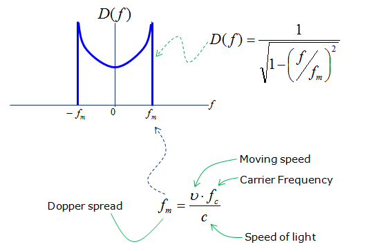
The last component I want to show you about Fading is Doppler spread. Doppler spread is caused by the well known phenomenon called 'Doppler Shift' (I would not explain what Doppler shift is. Everybody would learned about this from High school physics and you can easily google out a lot of explanation of this effect).
Doppler spread can be expressed as shown in following function and plot. If you think of 'Doppler spread' as a kind of filter (or a block in a control system model). You can take the following function as a kind of transfer function of the filter.
As you see, how much a frequency (fc) get spreaded by doppler spread is indicated by fm. If you see another formula below the graph representing fm, you would see fm is determined by the velocity of object (relative velocify between transmitter and reciever) and speed of light and fc(carrier frequency). You know fc is constant (set by standard and assume hardware is good enough to maintain the fc the same). Now the only variable is the speed v. According to this equation, fm and v are in proportional relation, meaning if v gets higher, fm gets larger (the width of the graph gets wider) and if v gets smaller, fm gets smaller (the width of the graph gets narrower).
How this kind of plot is obtained ? What is the meaning of this plot. Let's think a little bit further into how we get this plot.
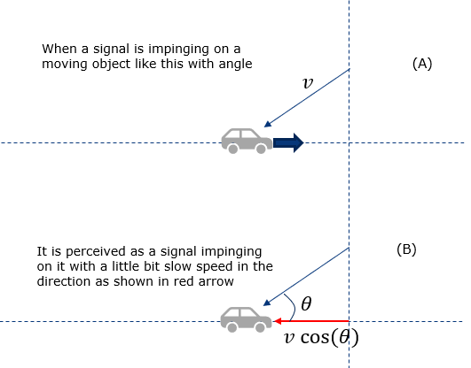
Let's assume that a car (e.g, a phone in a car) is moving in horizontal direction and it is receiving a signal with an angle illustrated as in (A). Since the car is moving, the phone in the car would experience doppler shift. Since the UE is getting the signal with an angle, the doppler shift it percieves can be represented as in red arrow in (B).
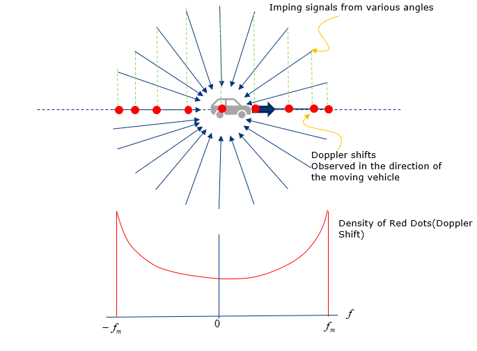
Now let's extend this situation further to the situation where the UE in the moving car is receiving the signal from all direction as illustrated below. This is the situation where the UE has so many reflectors around it and recieves the multipath signal all around. Then the doppler shift that UE percieves is like red dots marked on the horizontal line. If you plot those red dots in probability distribution function, you will get the red plot as shown below.
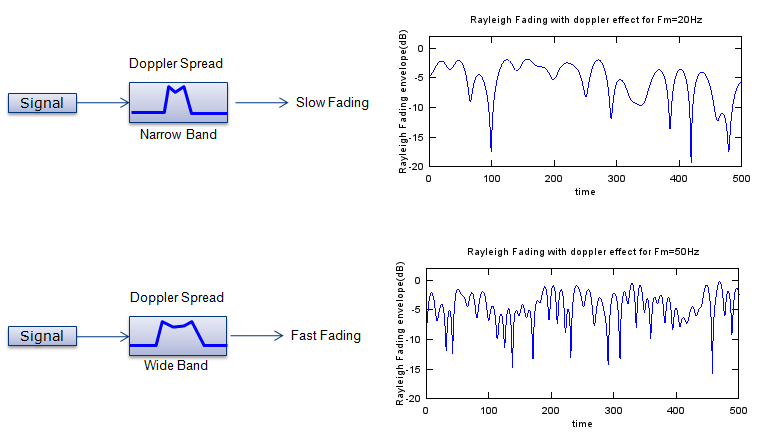
Now you may have question. How differently the narrow Doppler spread and wide doppler spread affect on the signal ?
The simulation result for these two cases (narrow and wide doppler spread) is shown below. The upper track is for narrow doppler spread and the lower track is for wide doppler spread. As you see, you see much frequency energy fluctuation over time in wide Doppler spectrum. I will update the page later about the mathmatical background.
High Speed Train Model (Scenario)
If you are using a phone in high speed train, the distance between UE and eNB changes very fast. It means both UE and eNB will be under drastic doppler shift.
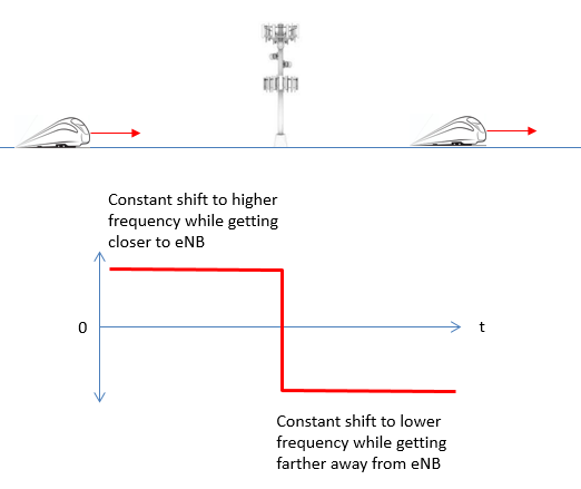
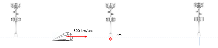
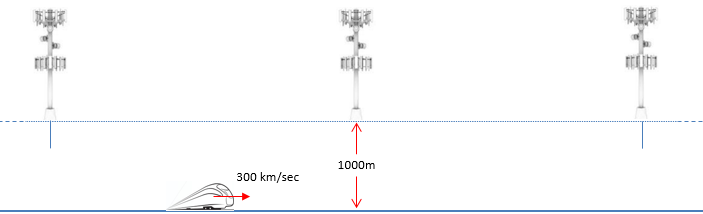
For example, let's suppose the train is traveling right into the eNB as illustrated below (the eNB is right on top of the railway). Of course, you don't see this kind of situation in real life. The train will crash into the eNB in this case. However, just suppose this is possible and train can go through a ghost-like eNB. In this case and assume that the speed of the train is constant, the doppler shift will stay constant as well. The only change is the direction of frequency shift changes as the train pass through eNB as illustrated below.
However, in realy you don't see any case shown above in real life. In real life, the eNB is located away from the rail way at certain distance.
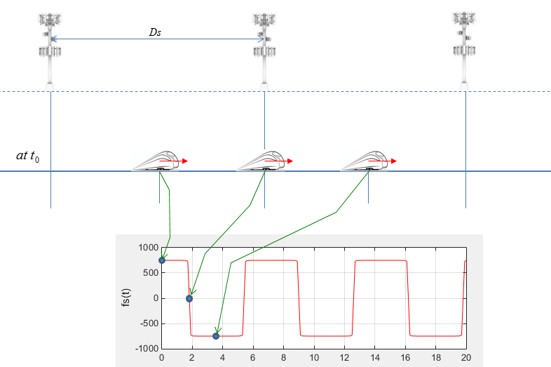
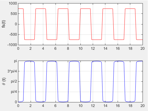
In this case, the Doppler Shift changes as the train get closer to, pass by and farther away from the eNB. The doppler shift at a specific time is represented as shown below (36.101 B.3)
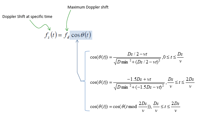
Where does this equation come from ? It turned out to be from hunior high school geometry, but it took me long time to understand this since there is no background information in 3GPP.
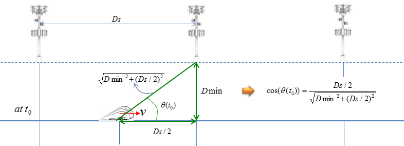
This model is based on the assumption that the eNBs are spaced equaly and the train moves at a constant speed. It is also assumed that the initial location of the train (the location at t = 0) on the railway is at the mid point between two adjacent eNBs as shown below. Dmin is defined as the closest possible distance between UE and eNB and the initial location is specified to be half way between two adjacent eNBs. Then, the distance between the eNB and the train can be derived. If we define the angle theta as shown below, the cos(theta) will become as below.
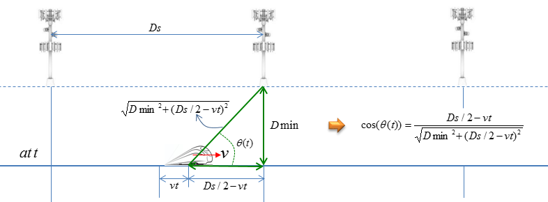
Now let's look into a snapshot after t seconds. Now the location of the train on the railway and the distance between UE and eNB, and the cos(theta) is derived as shown below. (Just try to derive on your own or just copy it with a pen on a paper, you will understand it clearly).
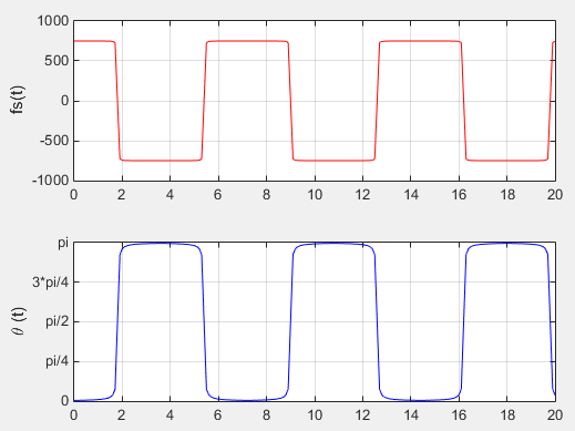
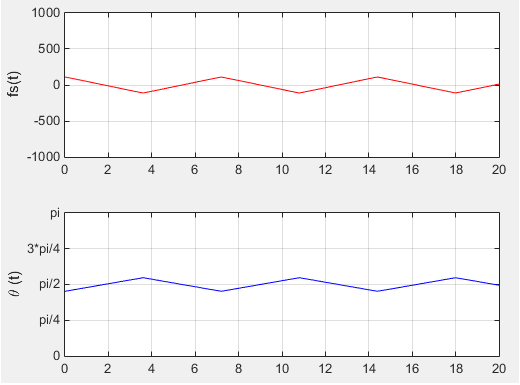
If you plot the doppler shift with time as traing travel along the railway, it would be illustrated as shown below.
Following is the Matlab code that I wrote based on the equation shown above. In this, I calculated not only frequency shift but also the angle(theta) to figure out the location of the train more easily.
function main
fd = 750;
Dmin = 2; % in meter
Ds = 300; % in meter
v = 300 * 1000/3600; % in m/s
tmin = 0;
tmax = 20;
tstep = 0.1;
fs = [];
th = [];
for t = tmin:tstep:tmax
costh = CosTh(t,Dmin,Ds,v);
y = fd .* CosTh(t,Dmin,Ds,v);
fs = [fs y];
th = [th acos(costh)];
end
subplot(2,1,1);
plot(tmin:tstep:tmax,fs,'r-');
xlim([tmin tmax]); ylim([-1000 1000]);
ylabel('fs(t)');
grid();
subplot(2,1,2);
plot(tmin:tstep:tmax,th,'b-');
xlim([tmin tmax]);
ylim([0 pi()]);
set(gca,'ytick',[0 pi/4 pi/2 3*pi/4 pi]);
set(gca,'yticklabel',{'0', 'pi/4', 'pi/2', '3*pi/4', 'pi'});
ylabel('\theta (t)');
grid();
end
function y = CosTh(t, Dmin, Ds, v)
if (t >= 0) && ( t <= Ds / v)
y = (Ds ./ 2 - v .* t)/sqrt(Dmin .^ 2 + (Ds ./ 2 - v .* t)^2);
elseif (t > Ds / v) && ( t <= (2 .* Ds ./ v))
y = (-1.5 .* Ds + v .* t)/sqrt(Dmin .^ 2 + (-1.5 .* Ds + v .* t)^2);
elseif (t > 2 .* Ds ./ v)
y = CosTh(mod(t, 2 .* Ds ./ v),Dmin, Ds, v);
end
end
Following is the result of the execution with the condition as defined below.
fd = 750;
Dmin = 2; % in meter
Ds = 300; % in meter
v = 300 * 1000/3600; % in m/s
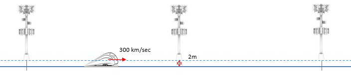
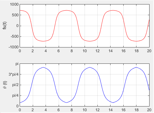
Now let's do some experiment with the code to understand the impact of the parameters. The first experiment is to change the speed of the train keeping all other parameters same. The doppler shift that UE (on the train) will experience can be plotted as shown below. See if this is aligned with your intuitive understanding.
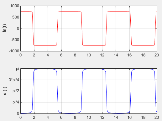
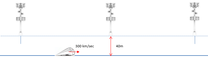
Now let's do another experiement. In this experiement, I changed Dmin keeping all other parameters same. The doppler shift that UE (on the train) will experience can be plotted as shown below. See if this is aligned with your intuitive understanding.
General Concept of Fading Channel Simulation
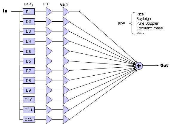
Typical model for Fading channel can be described by a simple diagram as follows. This is very simplified model but fortunately this is almost enough for 3GPP specification for fading test. As you see, a signal comes into the fading block and splits into multiple path. Each path has three components, namely Delay, PDF, Gain component. By changing these parameters in each path, you can construct pretty complicated fading channel.
In LTE 3GPP specification, typical three types of Fading profiles are defined as follows.
Go through following pages (examples) and try to get some intuitive understanding on your own.
- Rayleigh Channel (Description, Matlab Example)
- Rician Channel(Description, Matlab Example)
Reference
[1] Multipath and Doppler Effects and Models
[2] Rayleigh Fading Channels in Mobile Digital Communication Systems. Part 1 : Characterization
Bernard Sklar, Communications Engineering Services.
IEEE Communications Magazine, July 1997
[3] Building High SPEED by Huawei
[4] Wireless Channel Modeling - Clarke's, Jakes' and modified Jakes' models
[5] Mobile Radio Channels Modeling in MATLAB
[6] MODELLING AND SIMULATION OF A FADING CHANNEL
[7] Simulation of Rayleigh Fading ( Clarke’s Model – sum of sinusoids method)
YouTube
[3] Wireless Communications: Small Scale Fading