'Least Square' is a special type of technique for data regression based on 'Sum of square of error between the given data and the estimated function(regression equation).

Does this make sense to you ?

Don't worry if this does not make sense to you. It doesn't make sense to me either :)

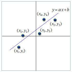
Let's take more practical (intuitive approach). Let's assume that somebody gave you the following 5 data points in the form of (x(n),y(n)) which can be plotted as shown below and he ask you to find a single straight line (a linear function) that can best represent (best fit) the whole data set. I assume that everybody would understand the linear function can be expressed as y = a x + b (this is a function from junior highschool math). You can change the location and the slope of the line (blue line in the following plot) by applying various different value for 'a' and 'b'.

Now the question become 'How can you figure out the value for 'a' and 'b' to make the line best fit for the given data set ?'.

Do you have any idea ?

The first idea you can think of is just try random values and keep doing 'try and error'.

Of course, this is not the one I would recommend. But I suggest you to do random trial at least several times and then you will understand why we need some kind of mathematical approach and will be highly motivated to follow the mathematical procedure all the way to the end even though sometimes it would be hard and sometimes (actually most of times) it become very boring.

There are largely two kinds of methods that are commonly used for this problem. One is 'Calculus' based and the other one is Matrix (linear algebra) based method.

• Calculus Method
• Matrix Method
• Why does the normal equation give the least square error?

Calculus Method

Let's start with the method that needs only high school calculus. The idea is to turn "best fit" into one number that you can minimize. Once the error of the whole data set is a single function of a and b, finding the best line becomes finding the lowest point of that function.

Basic idea of this method is

• i) Figure out an equation representing error between the each real data point (data point given to you) and the estimated data point (data point on the estimated line y = a x + b). You will get as many error equation as the given data points.
• ii) Get each of the error equations squared.
• iii) Sum up all the squared error equation (at this step, you will have a long/complicated quadratic function with variable 'a' and 'b'.
• iv) Find the value of 'a' and 'b' that gives you the minimum of the quadratic function.

As a first step, let's look at how 'error' for each data point are defined. The error for each data is defined as shown below. The red point is the estimated point (the ideal data points when we assumed that the regression line is y = a x + b) and the blue point is the data that are given to us.

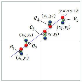
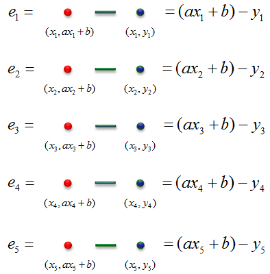
Error for each data point is the difference between the red point and blue point. Equation of error for each data point obtained by this method are as follows,

Once we have all these error equation, the goal is to find 'a' and 'b' that satisfy the following condition. (As you see, this is to find the least point of sum of squared error. That's how the term 'Least Square' came from).

At this point, you may ask why we need to get all the error squared. Why not simply adding up all the errors as follows without squaring.

This cannot be used because in some case just summing up the errors would give you completely wrong information. For example, let's assume that you have error is 100 and another error = -100. It is pretty big error and the only difference is the direction of the error and only sign of th evalue is different. But if you sum up these two errors as they are, it gives you the result of '0' (e1 + e2 = 100 + (-100) = 0) that may give you the impression that there is no error at all.

Then you may ask why not using following equation. This would resolve the issue that is mentioned above. It is true. It can solve the problem that a negative error is canceled away with a positive error. But this absolute equation is hard to analyze mathematically (especially with Calculus).

Now I think we all understand why we need to use 'Squared Sum of Errors' as follows.

If you plug in each error equation into the equation above, you would get the following equation. It would look scary, but it can be done by high school math. Just don't get scared and try on your own.

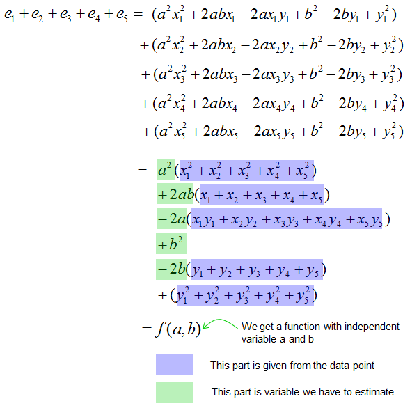
If you have a real data value for x(n) and y(n) and plug all those values into the equation shown above. You will have a quadratic equation with two variable 'a' and 'b' and you can plot the quadratic equation as shown below.

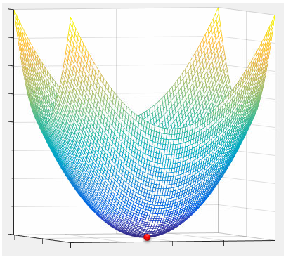
Now the problem become 'find the value 'a' and 'b' marked in the red dot shown above and it is the point that is the minimum value point of the quadratic plot'.

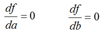
As you learned from High school math (Pre-Calculus or Calculus), it is the point where it satisfies the following condition.

I would not solve this equation any further since the important thing is how you come to this point and meaning of this point. In reality, finding the point would be done by various computer software.

Three details in the pictures above need a careful reading before you solve anything. First, the expansion writes e₁ + e₂ + e₃ + e₄ + e₅ on its left side. The right side, however, is the expansion of e₁² + e₂² + ... + e₅², so read the left side as the sum of squared errors. Second, each of the five brackets carries its own b². The grouped term "+b²" should therefore be +5b², or +nb² for n data points. Third, f depends on both a and b, so df/da and df/db are partial derivatives. Each one is taken with the other variable held fixed.

Let's finish the step that was left open above. With n data points, the function is f(a,b) = a²Σx_i² + 2abΣx_i - 2aΣx_iy_i + nb² - 2bΣy_i + Σy_i². Take the two partial derivatives and divide each by 2. The result is two linear equations in a and b, and they are called the normal equations.

∂f/∂a = 2aΣxi2 + 2bΣxi - 2Σxiyi = 0     which gives     aΣxi2 + bΣxi = Σxiyi
∂f/∂b = 2aΣxi + 2nb - 2Σyi = 0     which gives     aΣxi + nb = Σyi

The second equation is useful on its own. Divide it by n, and it becomes b = mean(y) - a x mean(x). So the best line always passes through the point (mean(x), mean(y)), which is the centre of the data. Put this b into the first equation, and you get the slope as a = Σ(x_i - mean(x))(y_i - mean(y)) / Σ(x_i - mean(x))².

You can check the equations on the five points of Example 1 below. The sums are Σx_i = -1, Σx_i² = 27, Σy_i = -3.4 and Σx_iy_i = 33.8, with n = 5. The two normal equations and their solution are:

27a -  b =  33.8
 -a + 5b =  -3.4

a = (5 x 33.8 - 3.4) / (5 x 27 - 1) = 165.6 / 134 = 1.2358
b = (a - 3.4) / 5                   = -0.4328

These are the same numbers that Matlab prints in Example 1, where x = [b; a] = [-0.4328; 1.2358]. The calculus method and the matrix method therefore reach the same answer in two different ways.

One question is still open. How do you know that this point is a minimum, and not a maximum or a saddle point? The second derivatives answer it. They are ∂²f/∂a² = 2Σx_i², ∂²f/∂b² = 2n and ∂²f/∂a∂b = 2Σx_i, and none of them depends on a or b. For the example they are 54, 10 and -2. The determinant 54 x 10 - (-2)² = 536 is positive, and 54 is positive too. So f is a bowl that opens upward, as the surface plot above shows. This holds for any data set, as long as the x values are not all the same. If every x_i is equal, the data sit on a vertical line, and no line of the form y = a x + b can describe them.

• Squaring keeps positive and negative errors from cancelling : it also gives a smooth function of a and b, so calculus can find its minimum.
• Two unknowns give two normal equations : setting ∂f/∂a = 0 and ∂f/∂b = 0 turns the search for the minimum into a 2 x 2 linear system.
• The best line passes through the centre of the data : the condition ∂f/∂b = 0 is the same as b = mean(y) - a x mean(x).
• The minimum is guaranteed unless all x values are equal : the error surface is an upward bowl with a single lowest point.

Matrix Method

Another method to solve this problem (finding the regression equation) is to use Matrix (Linear Algebra) equation. I would just put down the conclusion of this method and would not go through the detailed 'Proof' and 'Derivation' process.

In real situation, this method would be more widely used comparing to 'Calculus' method described above. Also, in most case you would use various kinds of software to find the solution. Most of the real life problem will generate pretty big matrix which is hard to be solved by pen-and-pencil.

However, at least you need to know how to construct the matrix equation itself from the given data set even though the calculation process is done by software.

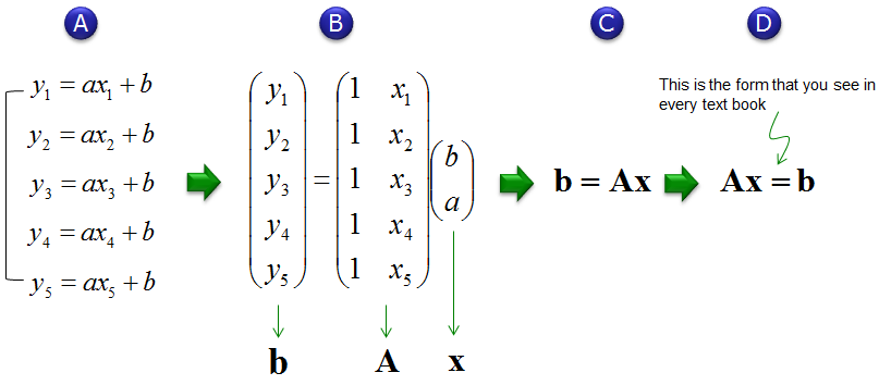
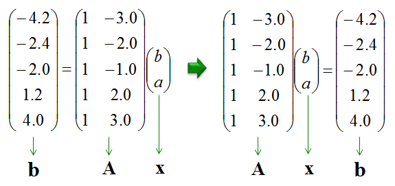
From the given data set and the regression equation that we want to fit the date to (y = a x + b in this example), you can generate equations as shown in (A). And then you can convert the simultaneous equation to a matrix equation as (B). (Refer to Matrix : Simultaneous Equation page if you are not familiar with this conversion).

If you replace the matrix and vector with a character just to make it simple (look less scary), you would get the equation as shown in (C) and (D) which you would see in most of linear algebra textbook.

Once you get a Matrix Equation as shown above, you can apply the techniques you would learn from most of Linear Algebra textbook.

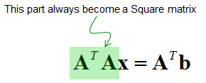
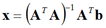
By muliplying transpose (A) on both side, you can rewrite the equation as below.

Also applying the simple algebric rule, you can find the solution (the vector x) as shown below.

You may have a question "I understand how I got the vector x in this process, but I don't understand how we can guarantee the 'x' obtained in this process will be the value that minimized the error (the error between the given data and the corresponding the point on regression line).

Very good question. But I would not go through the details of this. You may find the answer from many textbook or even just by googling.

Example 1

Just to give you clearer understanding. I would give you an example. I used Matlab in this example, but I used very small number of data set so that you can even try with pen-and-pencil on your own.

Let's assume that you have following data set which is made up of 5 data points.

{(x1,y1), (x2,y2), (x3,y3), (x4,y4), (x5,y5)} = {(-3, -4.2),(-2, -2.4),(-1.0,-2.0),(2.0,1.2),(3, 4.0)}

The first step is to generate a matrix equation from this dataset. I strongly suggest you to construct this matrix equation on your own in hand writing.

If you get the matrix equation as shown below, you did it right. One very important thing is to keep remind you of the meaning of each elements in each matrix and vectors. Especially the meaning of 'b' and 'a' in the vector 'x'. Otherwise, you would not know how to interpret the result when your software gives you the result of the calculation. In this case, 'b' is the 'y intercept' of the regression equation and 'a' represents the slope of the regression equation.

Once you get this matrix equation, you can use any software that you like to solve the equation. I used Matlab here and following is the matlab code for this.

p = [-3 -4.2;-2 -2.4;-1.0 -2.0;2.0 1.2;3 4.0];

A = [1 p(1,1);1 p(2,1);1 p(3,1);1 p(4,1);1 p(5,1)]
b = p(:,2)
x = (inv(A' * A) * A') * b % this gives you to solution of the matrix equation.

% This part is not mendatory process, but I just put this to draw a plot to show you how well the solution fits 
% the given dataset.

t = -5:1:5;
y = x(2)*t + x(1);

plot(p(:,1),p(:,2),'bo',t,y,'r-'); 
axis([-5 5 -5 5]);

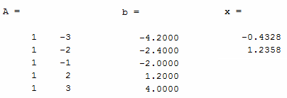
Following is the numerical result. Actually A, b is the one I manually set in the code (this is a kind of input) and only the vector 'x' is the calculated value (this is the output)

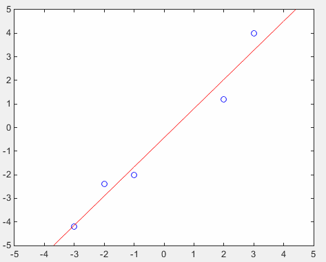
Following is the graph showing both  given data set and the regression line. Blue points are the given data and the red line is regression line.

Let's read the result with the meaning of each element in mind. The vector x is [b; a], so x(1) = -0.4328 is the intercept and x(2) = 1.2358 is the slope. That is why the plotting code writes y = x(2)*t + x(1). The fitted line is therefore y = 1.2358x - 0.4328. It crosses the y axis just below zero and rises by about 1.24 for each step of 1 in x, which matches the red line in the plot above.

The line does not pass through any of the five points exactly. The residuals y_i - (a x_i + b) are -0.060, 0.504, -0.331, -0.839 and 0.725. Their sum is zero, and the sum of their squares is 1.598. No other choice of a and b gives a smaller sum of squares for this data set. The coefficient of determination is R² = 0.962, so the line explains about 96 percent of the variation in y.

The code computes the solution as inv(A' * A) * A' * b, which is the textbook formula written directly. It gives the right answer here. For larger or badly scaled problems, x = A\b is the safer choice in Matlab. The backslash operator solves the least square problem with a QR decomposition and never forms A^TA. This matters because the condition number of A^TA is the square of the condition number of A.

• Each data point becomes one row of A and one entry of b : a straight line fit gives a column of ones for the intercept and a column of x values for the slope.
• The order of the unknowns decides how you read the result : with x = [b; a], the first output is the intercept and the second output is the slope.
• The bold b and the italic b are different things : the vector b holds the measured y values, while the scalar b is the intercept inside x.
• Prefer A\b to inv(A'*A)*A'*b in code : both give the least square solution, but the backslash operator is more accurate on ill-conditioned data.

Why does the normal equation give the least square error?

The Matrix Method above leaves one question open. Multiplying both sides of Ax = b by A^T looks like a simple algebra trick, so why should its result be the best fit? Let's answer it in two ways. The first way uses the same calculus as the Calculus Method. The second way uses a picture, and it explains why least square is often called a projection.

Start with the reason why Ax = b needs any trick at all. In Example 1, A has 5 rows and 2 columns, so the system has five equations and only two unknowns. The five points do not lie on one line, so no x satisfies all five equations at once. Instead, we define the error vector e = Ax - b and look for the x that makes its squared length as small as possible.

E(x) = eTe = (Ax - b)T(Ax - b)
     = xTATAx - 2xTATb + bTb

gradient of E = 2ATAx - 2ATb = 0     which gives     ATAx = ATb

This is exactly the equation of the Matrix Method. So multiplying by A^T is not a trick. It is the condition that the gradient of the squared error is zero. It is also the same pair of equations as in the Calculus Method, and the products for a straight line fit show this directly:

ATA = [ n , Σxi ; Σxi , Σxi2 ]          ATb = [ Σyi ; Σxiyi ]

Example 1 :  ATA = [ 5 , -1 ; -1 , 27 ]          ATb = [ -3.4 ; 33.8 ]

The first row is the condition ∂f/∂b = 0, and the second row is ∂f/∂a = 0, because x lists b before a. E(x) is the same function as f(a,b), so its Hessian 2A^TA describes the same upward bowl. A^TA is invertible when the columns of A are linearly independent. For a line fit, that means the x values are not all equal.

The second answer is geometric, and Figure 1 draws it. Every product Ax is a combination of the two columns of A. So all the vectors Ax form a plane inside the 5-dimensional space of b. This plane is the column space of A. The measured vector b sits outside the plane. The point of the plane closest to b is the foot of the perpendicular from b. That point is Ax_LS, the orthogonal projection of b onto the plane, where x_LS is the least square solution.

Figure 1. Least square as a projection. The residual b - Ax_LS meets the column space of A at a right angle, and A^T(b - Ax_LS) = 0 is the normal equation.

• The plane holds every possible fit : each choice of a and b gives one vector Ax of fitted y values, and all of them lie in the column space.
• The dashed line is the residual : its squared length is the sum of squared errors, and it is shortest when it meets the plane at a right angle.
• A right angle to the plane means a right angle to each column : A^T(b - Ax_LS) = 0 states exactly that, and it rearranges to A^TAx_LS = A^Tb.

The right angle has a practical consequence that you can check on Example 1. The first column of A is all ones, so the residuals r_i must add up to zero. The second column holds the x values, so Σx_ir_i must also be zero. With the residuals -0.060, 0.504, -0.331, -0.839 and 0.725, both sums are zero to within rounding. Any fit with an intercept column has a zero mean residual for the same reason.

The same algebra works for any model that is linear in its unknowns. A parabola y = c₀ + c₁x + c₂x² only adds a third column of x_i² values to A. The normal equation, the projection picture and the zero sum of the residuals all stay the same.

• A^TAx = A^Tb is the zero-gradient condition : it is the matrix form of the two calculus conditions ∂f/∂a = 0 and ∂f/∂b = 0.
• Least square is an orthogonal projection : the fitted values Ax_LS are the point of the column space that is closest to b.
• The residual is perpendicular to every column of A : with an intercept column, the residuals therefore always sum to zero.
• The solution is unique when the columns of A are linearly independent : otherwise A^TA is singular, and many x give the same smallest error.