As you may know, Matrix would be the tool which has been most widely studied and most widely used in engineering area. So if you can convert any mathemtical expressions into a matrix form, all of the sudden you would get the whole lots of the tools at once.

So it would be a very meaningful to ask following question :

i) Is it possible to convert a certain form of differential equation into a matrix form ?

ii) If the answer to question i) is YES, is it possible to convert ANY differential equations into a matrix form ?

iii) If the answer to question ii) is "Not ANY, but SOME", what kind of differential equations can be converted into Matrix form ?

The answer to the question i) is YES.

The answer to the question ii) is "NOT Always"

The answer to the question iii) is "Linear Homogeneous Differential Equations" or "Linear Non-Homogeneous Differential Equation". (Basically Matrix itself is a Linear Tools. That's why you learn it at "LINEAR Algebra course" -:)

Isn't there any way to use Matrix to solve Non Linear Homogeneous Differential Equation ? It is not possible as it is, but if you can convert the Non Linear Equations into a linear equation (Basically this is a approximation within a certain range of domain), it would be possible to use Matrix (I will explain on this 'linearization' process later in other section).

• How is a set of simultaneous differential equations written as a matrix?
• How does a higher order differential equation become a matrix equation?
• How is a non-homogeneous equation written in matrix form?

How is a set of simultaneous differential equations written as a matrix?

Let's look into the details of the process to convert a differential equation into a matrix form. As you would have learned in Matrix pages, you would need a set of simultaneous equations to construct a matrix. In this case, you would need a set of simultaneous differential equations to construct a matrix.

Let's suppose we have a set of simultaneous differential equations as follows. (This is a form of linear homogeneous simultaneous equations). For now, let's not think about the meaning of these equations.. let's just suppose it's given to us. (Note that y1, y2 here are function of x, it is not a value. It is a function which can be represented as y1(x), y2(x))

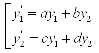
You can easily notice that this simultaneous equations can be converted into following matrix form.

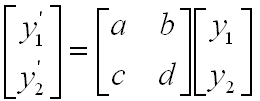
You can simplify this representation even further as shown in the following process. At the end you would have very simple equation y' = A y. This simplified form would look very nice in mathematically, but it looks scary to a lot of readers if you don't know the detailed process of how these equations were derived).

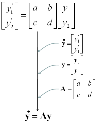
Check the vector definitions on the right side of the diagram above. The second entry of y' should read y₂', and the second entry of y should read y₂. The diagram repeats y₁' and y₁ there by mistake. The matrix equation at the top and the compact result at the bottom are correct.

Once you have a set of differential equations represented in Matrix form, you can use a lot of powerful Matrix tools to solve the problem. I will just write the final form of solutions of this form. The solution of this matrix equation is presented as follows. As you see, a special matrix analysis tool called "Eigenvalues" and "Eigenvectors" are used to describe the solution of the differential equation. Sometimes it would be pretty complicated to calculate Eigenvalues and Eigenvectors especially as the size of the matrix gets bigger and very large portions of your text book tend to get thicker because they try to explain a lot of this calculation process, but I would not explain anything about how to calculate "Eigenvalues" and "Eigenvectors" because you can easily get these values using Matlab, Octave, Mathematica etc and in reality almost nobody would calculate these values by hand). Important thing is to understand the mathematical expression as shown below. Even this, it would be a little difficult to have intuitive understanding without have some concrete examples, but I would add some examples later... for now at least try to understand the meaning of this form based on what you understand about Eigenvalues and Eigenvectors.

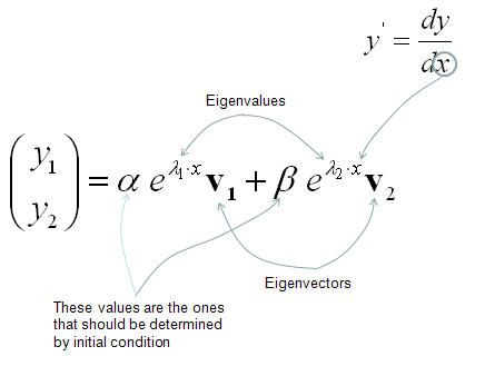
Let's read this solution term by term. Each eigenvalue λ_i of A gives one exponential e^λ_ix, and its eigenvector v_i fixes the direction of that term in the y₁-y₂ plane. You can check one term directly. Suppose y = e^λxv and Av = λv. Then y' = λe^λxv = e^λxAv = Ay, so each term solves the equation on its own. The equation is linear, so any combination of the two terms, with constants α and β, solves it too. The two constants α and β are then fixed by the two initial values y₁(0) and y₂(0).

The eigenvalues also tell you how the system behaves before you compute anything else. A negative real eigenvalue gives a term that decays to zero. A positive real eigenvalue gives a term that grows without limit. A complex pair λ = σ +/- jω gives an oscillation at the angular frequency ω, inside the envelope e^σx. This is why engineers check the eigenvalues of A first when they ask whether a system is stable.

One warning goes with this form. It needs two independent eigenvectors, and that is guaranteed when the two eigenvalues are different. Sometimes A has a repeated eigenvalue λ with only one eigenvector v. In that case the second term becomes e^λx(xv + w), where w solves (A - λI)w = v. The solution shown above does not cover that case as written.

• A linear system of first order equations becomes y' = Ay : Each row of A holds the coefficients of one equation, in the same order as the entries of y.
• Eigenvalues give the exponents and eigenvectors give the directions : The solution is a sum of terms e^λxv, one for each eigenvalue and eigenvector pair of A.
• The initial values fix only the constants : α and β come from y(0). The eigenvalues and eigenvectors depend on A alone.
• The sign of the real part decides stability : Every eigenvalue with a negative real part gives a decaying term. One eigenvalue with a positive real part is enough to make the solution grow.

How does a higher order differential equation become a matrix equation?

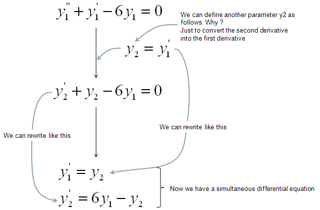
You may think this matrix form would not be useful in many case since there would not be many cases where we have a set of simultaneous equations. But it is not true. Actually this kind of simultaneous differential equations are very common. Sometimes it is given directly from modeling of a problem and sometimes we can get these simultaneous differential equations by converting high order (same or higher than 2nd order) differential equation into a multiple of the first order differential equations. Following is one example of this case.

Let's suppose we have a following 2nd order linear homogeneous differential equation.

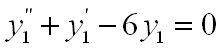
You can get a set of simultaneous differential equation being made up of two first order linear homogeneous differential equations. I hope that following illustration would be explicit enough.

Once you have this multiple equations, you can easily convert it into a matrix forma as follows.

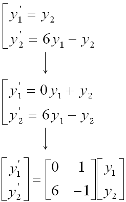
Let's finish this example, because the matrix is not the end of the work. The matrix A = [0 1; 6 -1] has the characteristic equation λ² + λ - 6 = 0. Its roots are λ₁ = 2 and λ₂ = -3. The matching eigenvectors are v₁ = [1, 2]^T and v₂ = [1, -3]^T. Put these into the solution form of the previous section, and you get y₁(x) = αe^2x + βe^-3x and y₂(x) = 2αe^2x - 3βe^-3x.

Now compare the characteristic equation with the original equation y₁'' + y₁' - 6y₁ = 0. If you try y₁ = e^λx directly in it, you get the same polynomial λ² + λ - 6 = 0. This is not a coincidence. A matrix built this way is called the companion matrix of the equation. Its eigenvalues are always the roots of the characteristic polynomial of the original equation. The eigenvectors also follow a pattern. The second entry of each eigenvector is λ times the first entry, because y₂ is defined as y₁'.

For a concrete case, take y₁(0) = 1 and y₁'(0) = 0. The two conditions give α + β = 1 and 2α - 3β = 0, so α = 3/5 and β = 2/5. The e^2x term grows, so this solution grows without limit. Only the initial values with α = 0 give a decaying solution. The same recipe works for any order. An n-th order linear equation needs n state variables y, y', ..., y^(n-1), and it gives an n x n matrix.

• One new variable per derivative : An n-th order equation becomes n first order equations, and the matrix is n x n.
• The companion matrix keeps the characteristic equation : Its eigenvalues are the roots of the original equation, here 2 and -3.
• Only the last row carries the equation : The first row [0 1] only says y₁' = y₂. The last row holds the coefficients of the original equation with their signs changed.

How is a non-homogeneous equation written in matrix form?

There is another type of linear differential equation which is linear non-homogenous differential equation. As I mentioned at the beginning of this section, it is also possible to convert this into a matrix form.

Let's assume that we have a set of simultaneous differential equation as follows.

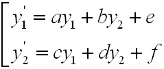
You know that this set can be represented in Matrix form as follows.

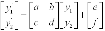
You can simplify this even further by the following process. You don't need this simplification if you don't like, but it is good to know at least since many literature use this kind of simplified form.

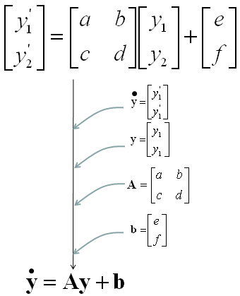
Check the vector definitions on the right side of the diagram above. The second entry of y' should read y₂', and the second entry of y should read y₂. The diagram repeats y₁' and y₁ there by mistake. The matrix equation at the top and the compact result at the bottom are correct.

The solution of this form can be expressed as follows. As you see, most part is exactly same as homogenous case. there is one additional term at the end.

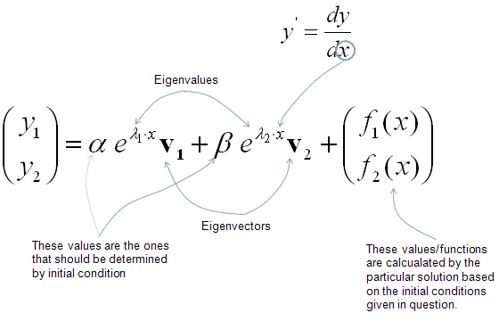
Let's be precise about the last term, because the note in the diagram above mixes two things. The last term is a particular solution, which means any one function that satisfies y' = Ay + b. It does not depend on the initial conditions. The initial conditions enter only through α and β, and you fit them after the particular solution is added. When e and f are constants and A is invertible, the particular solution is a constant vector. Set y' = 0, and you get Ay_p + b = 0, so y_p = -A^-1b.

For example, add b = [0, 6]^T to the system of the previous section. This corresponds to y₁'' + y₁' - 6y₁ = 6. Then y_p = -A^-1b = [-1, 0]^T. You can check it in the original equation, because y₁ = -1 gives 0 + 0 + 6 = 6. The full solution is y₁(x) = αe^2x + βe^-3x - 1, and the eigenvalues are the same as before.

Sometimes e and f are functions of x rather than constants. Then the particular solution is not a constant either. The general formula uses the matrix exponential: y(x) = e^Axy(0) + ∫₀^x e^A(x-s)b(s) ds. The first part is the homogeneous solution of the first section, written in compact form. The integral is one particular solution, and it is zero at x = 0.

• A non-homogeneous system is y' = Ay + b : The vector b collects every term that does not multiply y₁ or y₂.
• The homogeneous part does not change : The eigenvalues, the eigenvectors and the stability are the same as for y' = Ay.
• The particular solution does not use the initial conditions : For a constant b it is the equilibrium -A^-1b. α and β are fitted afterwards.