An analytic solution is a formula for y, found by hand with algebra and integration. Only some equations have one, and each solvable type has its own recipe. So the first step is always to recognize the type. This page is an index. It lists three common patterns with a solution guide for each, and then example and application problems that use them. Each link opens a worked solution on its own page.

• Patterns
• Example Question and Solution
• Application Problem and Solution

Patterns

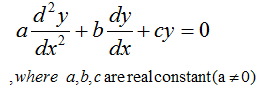
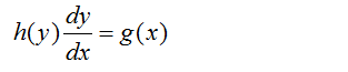
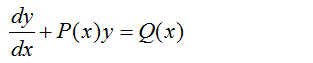
Let's start with the three patterns, because every problem further down reduces to one of them. Pattern 1 is a separable equation: all y terms go to one side and all x terms to the other, and you integrate both sides. Pattern 2 is a linear first order equation, solved with the integrating factor e^∫P(x)dx. Pattern 3 is a linear second order equation with constant coefficients and zero right side. Its solution comes from the roots of the characteristic equation ar² + br + c = 0.

Pattern 1		Solution Guide
Pattern 2		Solution Guide
Pattern 3		Solution Guide

Example Question and Solution

Each example below is a direct use of one pattern. Before you open a solution, try to name the pattern yourself. Examples 1 and 2 can be solved with Pattern 1 or Pattern 2. Example 3 needs Pattern 2, and Example 4 is Pattern 3.

(1) Solve		Solution
(2) Solve		Solution
(3) Solve		Solution
(4) Solve		Solution

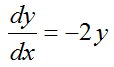
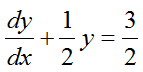
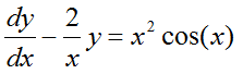
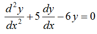
You can check your own answers against these general solutions. They were verified by substituting them back into each equation. Example 1 gives y = Ce^-2x. Example 2 gives y = 3 + Ce^-x/2. Example 3 has the integrating factor x^-2, and it gives y = x²sin(x) + Cx². In Example 4 the characteristic equation r² + 5r - 6 = 0 has the roots 1 and -6, so y = C₁e^x + C₂e^-6x.

Application Problem and Solution

These problems start from a physical or economic situation rather than from a given equation. The modeling step has already been done, and each equation is first order. Most of them have the form y' = ay + b, so they are Pattern 1 and Pattern 2 at the same time.

(1) Solve		Population Problem	Solution
(2) Solve		Population Problem	Solution
(3) Solve		Mixing Problem	Solution
(4) Solve		Free Fall	Solution
(5) Solve		Finance : Saving	Solution

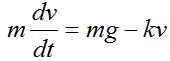
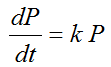
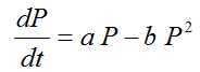
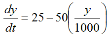
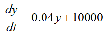
A useful check for this kind of model is the equilibrium, the value where the derivative is zero. The exponential population model gives P = P₀e^kt and has no nonzero equilibrium. The logistic model aP - bP² levels off at P = a/b. The mixing tank settles at y = 500, since 25 - 50y/1000 = 0 there, with the time constant 20. The falling body reaches the terminal velocity v = mg/k. The saving account y' = 0.04y + 10000 has the solution y = Ce^0.04t - 250000, which grows without limit for any start value above -250000.

• Find the pattern first : Separable, linear first order and constant coefficient second order cover every problem on this page.
• y' = ay + b is the most common model : Its solution is Ce^at - b/a. It approaches -b/a when a < 0, and it grows without limit when a > 0 and C is not zero.
• Check the answer by substitution : Put the solution back into the equation. The equilibrium value is a quick second check.