|
|
||
|
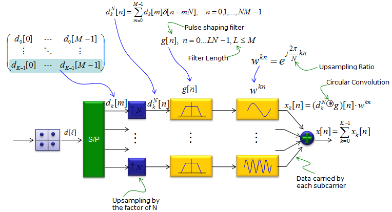
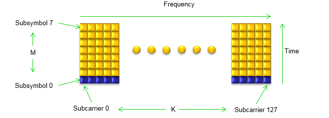
GFDM is also based on filtering method for each subcarrier. One important characteristic would be that the multiple symbol (subsymbols) across the whole frequency span is processed in a single processing unit. Basic concept and characteristics of GFDM is well explained in the video 5G Waveform Comparison from Anritsu as stated below. In this, we move from OFDM across, now we no longer orthogonal for every subcarrier, but we can change the characteristics of each sub carrier. So now we can actually interleave the different types of subcarrier. We can still have good spectral efficiency and good out of band emission and we can have MIMO support as well. This gives us very good flexibility, but we don't have good control of in-band emission or may be the spectral efficiency isn't so well improved as we can with other techniques. So it gives us more flexibility but less in terms of pure spectral efficiency improvement NOTE 1 : CP(Cyclic Prefix) - You may add CP if you need to make GFDM waveform more robust to inter symbol interference. But by design, only one CP is added at the beginning of a GFDM frame that is made up of multiple subsymbols. So the overhead created by CP will be much less comparing to the OFDM that is currently used. NOTE 2 : Filtering - Filtering also applies to single subcarrier level in frequency domain meaning it is very long filter in time domain. This is similar to FBMC case. Following is the illustration for GFDM from GFDM Interference Cancellation for Flexible Cognitive Radio PHY Design ([1]) In this scheme, a filter called Pulse Shaping Filter is applied per each sub carrier and multiple symbols per sub carrier are processed in a single step. (In this illustration, M indicates the number of symbols and K indicates the number of subcarriers)
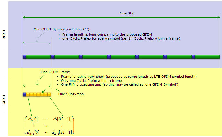
According to Ref [2], GFDM Frame structure can be compared to the current LTE structure as shown below. (The block diagram shown above may become clearer to you if you grasp the image of this frame structure first). As you see here, GFDM frame will be very short comparing to current LTE OFDM symbol to meet 5G latency requirement.
Following example code is from the code shared by Technical University Dresden (Refer to Ref 4 and see the full copyright description in the original source code) % Copyright (c) 2014 Technical University Dresden, Vodafone Chair Mobile % Communication Systems % All rights reserved.
clear all;
K=128;%number of subcarriers M=8;%number of subsymbols Kindex = 1:K;
r=0;%length of the cyclic prefix (CP) in multiples of 'subsymbols' CP=r*K; a=1;%roll-off
% Symbol source s = 1/sqrt(2)*(sign(randn(K,M))+1i*sign(randn(K,M)));%basic example s(:,1) = 0;%1st symbol null if r>0 s(:,M-r+1) = 0;end % M-r symbol null s([(K/8:3*K/8)+K/2],:) = 0;%some null subcarriers d=reshape(s,[K*M 1]);
% Split into real and imag di = real(d); dq = imag(d);
% Meyer RRC (defined in time) R=((0:(K-1))'-K/2-eps)/(a*K)+1/2;R(R<0)=0;R(R>1)=1;F=1-R;% Ramp rise/fall R=R.^4.*(35 - 84*R+70*R.^2-20*R.^3);F=1-R;% Meyer auxiliary function R=1/2*(cos(F*pi)+1);F=1-R;% Meyer RC rise/fall R=sqrt(R);F=sqrt(F);%Meyer RRC g=[F;zeros((M-2)*K,1);R]; g=g/sqrt(sum(g.^2));%normalization
% Frequency shift oqam gi = g; gq = ifft(circshift(fft(gi), M/2)); plot(real([gi gq]))
% Ai matrix Ai = zeros(M*K, M*K); n = 0:M*K-1; n=n'; w = exp(1j*2*pi/K); for k=0:K-1 for m=0:M-1 Ai(:,m*K+k+1) = 1i^(mod(m,2))*circshift(gi, m*K) .* w.^(k*n); end end
% Aq matrix Aq = zeros(M*K, M*K); for k=0:K-1 for m=0:M-1 Aq(:,m*K+k+1) = 1i^(mod(m,2)+1)*circshift(gq, m*K) .* w.^(k*n); end end
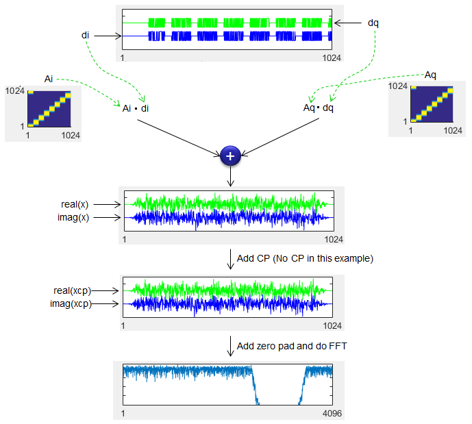
x=Ai*di+Aq*dq;
% Add CP xcp = [x([end-CP+(1:CP)],:);x];
Xcp=fft(xcp,4*M*K); Xcp=Xcp/std(Xcp);%normalize to ~0dB
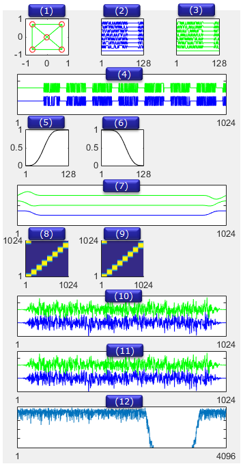
% Following code is what I added for analysis and visualization subplot(8,3,1); plot(real(s),imag(s),'g-',real(s),imag(s),'ro');
subplot(8,3,2); plot(Kindex,real(s(:,1))+2,'b-',... Kindex,real(s(:,2))+4,'b-', ... Kindex,real(s(:,3))+6,'b-', ... Kindex,real(s(:,4))+8,'b-', ... Kindex,real(s(:,5))+10,'b-', ... Kindex,real(s(:,6))+12,'b-', ... Kindex,real(s(:,7))+14,'b-', ... Kindex,real(s(:,8))+16,'b-'); axis([1 K 0 18]); set(gca,'yticklabel',[]); set(gca,'xtick',[1 K]);
subplot(8,3,3); plot(Kindex,imag(s(:,1))+2,'g-', ... Kindex,imag(s(:,2))+4,'g-', ... Kindex,imag(s(:,3))+6,'g-', ... Kindex,imag(s(:,4))+8,'g-', ... Kindex,imag(s(:,5))+10,'g-', ... Kindex,imag(s(:,6))+12,'g-', ... Kindex,imag(s(:,7))+14,'g-', ... Kindex,imag(s(:,8))+16,'g-'); axis([1 K 0 18]); set(gca,'yticklabel',[]); set(gca,'xtick',[1 K]);
subplot(8,3,[4 6]); dIdx = 1:length(di); plot(dIdx,di + 2,'b-', dIdx,dq+4,'g-'); xlim([1 max(dIdx)]);ylim([0 6]); set(gca,'yticklabel',[]); set(gca,'xtick',[1 max(dIdx)]);
subplot(8,3,7); plot(R,'k-'); xlim([1 length(R)]); set(gca,'xtick',[1 length(R)]);
subplot(8,3,8); plot(F,'k-'); xlim([1 length(F)]); set(gca,'xtick',[1 length(F)]);
subplot(8,3,[10 12]); gIdx = 1:length(gi); plot(gIdx,5*gi + 1,'b-', gIdx,5*real(gq)+2,'g-', gIdx,5*imag(gq)+3,'g-'); xlim([1 max(gIdx)]);ylim([0 4]); set(gca,'yticklabel',[]); set(gca,'xtick',[1 max(gIdx)]);
subplot(8,3,13); surf(abs(Ai),'EdgeColor','none'); xlim([1 size(Ai,1)]);ylim([1 size(Ai,2)]); set(gca,'xtick',[1 size(Ai,1)]); set(gca,'ytick',[1 size(Ai,2)]); view(0,90);
subplot(8,3,14); surf(abs(Aq),'EdgeColor','none'); xlim([1 size(Aq,1)]);ylim([1 size(Aq,2)]); set(gca,'xtick',[1 size(Aq,1)]); set(gca,'ytick',[1 size(Aq,2)]); view(0,90);
subplot(8,3,[16 18]); xIdx = 1:length(x); plot(xIdx,real(x) + 2,'b-', xIdx,imag(x)+4,'g-'); xlim([1 max(xIdx)]);ylim([0 6]); set(gca,'yticklabel',[]); set(gca,'xtick',[1 max(xIdx)]);
subplot(8,3,[19 21]); xcpIdx = 1:length(xcp); plot(xcpIdx,real(xcp) + 2,'b-', xcpIdx,imag(xcp)+4,'g-'); xlim([1 max(xcpIdx)]);ylim([0 6]); set(gca,'yticklabel',[]); set(gca,'xtick',[1 max(xcpIdx)]);
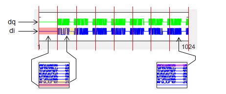
subplot(8,3,[22 24]); XcpIdx = 1:length(Xcp); plot(XcpIdx,mag2db(abs(Xcp))); xlim([1 max(XcpIdx)]);ylim([-80 10]); set(gca,'yticklabel',[]); set(gca,'xtick',[1 max(XcpIdx)]); Following is the subframe structure that this program is trying to modulate. Try to fully understand this structure and key variable name K, M. In this illustration, K and M is with the range of 0~7 and 0~127 respectively, but in Matlab it will be ranged as 1~8 and 1~128 because the array index in Matlab always start from 1.
Following is the result of the execusion showing each of the steps in procedure. Look into the source code and try to understand the meaning of each plot in the result. If you can make sense of these plots without further explanation, you don't have to read any further.
Now let's look at each plot and how these plots are related to the variables in the source code. The first plot shows the signal (variable s) in frequency and time domain. As you see, the original signal is constructed as a 2-D array.
Next step is to concatenate all the symbol (subsymbol) data into a long 1-D array as shown below. All the filtering and transformation will be applied to this 1-D array.
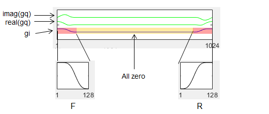
Next step is design the pulse shaping filter g. As the first step of designing the filter g, two components F and R are generated by using RRC filter equation. And then a long variable (gi) is created by concatenating F,zero pad and R as illustrated below. gq is generated by doing ifft of gi.
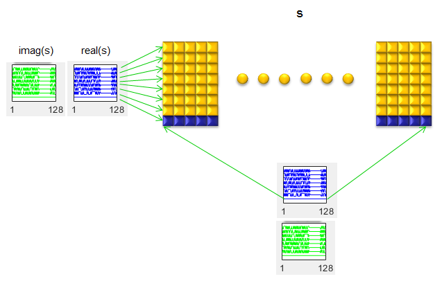
Next step is to generate a square matrix called A (Ai and Aq) by cyclic shifting the pulse shaping filter (gi, gq). Once the Ai and Aq are created, apply the filter and add CP and do FFT to get the final result as illustrated below.
Reference [1] GFDM Interference Cancellation for Flexible Cognitive Radio PHY Design R. Datta, N. Michailow, M. Lentmaier and G. Fettweis Vodafone Chair Mobile Communications Systems, Dresden University of Technology, 01069 Dresden, Germany Email:[rohit.datta, nicola.michailow, michael.lentmaier, fettweis]@ifn.et.tu-dresden.de [2] Designing A Possible 5G PHY With GFDM Gerhard P.Fettweis Ivan Gaspar, Luciano Mendes, Maximilian Matthe, Nicola Michailow, Andreas Festag, Rohit Datta, Martin Danneberg, Dan Zhang [3] Implementation Aspects of a GFDM-based Prototype for 5G Cellular Communications Ivan Simes Gaspar [4] Frequency-shift Offset-QAM for GFDM - Matlab script example by Technical University Dresden, Vodafone Chair Mobile Communication Systems Contact: ivan.gaspar@ifn.et.tu-dresden.de [5] Generalized Frequency Division Multiplexingfor 5th Generation Cellular Networks by Nicola Michailow, Maximilian Matth, Ivan Simes Gaspar, Ainoa Navarro Caldevilla,Luciano Leonel Mendes, Andreas Festag,Senior Member, IEEE, and Gerhard Fettweis,Fellow [6] Gerhard P.Fettweis - Designing A Possible 5G Framework With Generalized Freq. Division Multiplexing
|
||