This page is mainly for transport and physical layer process for PUSCH transmission. The overall procedure of the process are listed as below.
- DCI : Format 0_0, 0_1
- PUSCH Transport Process
- (1) Transport block CRC attachment
- (2) LDPC base graph selection
- (3) Code block segmentation And Code Block CRC Attachment
- (4) Channel Coding
- (5) Rate Matching
- (6) Code Block Concatenation
- (7) Data and control multiplexing
- (8) Scrambling
- (9) Modulation
- (10) Layer Mapping
- (11) Transform Precoding
- (12) Precoding
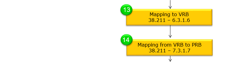
- (13) Mapping to VRB
- (14) Mapping from VRB to PRB
- RRC Parameters
PUSCH Transport Process
PUSCH transport process is performed in a long sequence of procedure as summarized below.
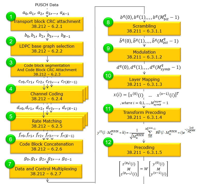
Following is brief summary for each step.
Transport Block CRC Attachment: Error checking codes are attached to the data.LDPC Base Graph Selection : The appropriate LDPC graph is selected for channel coding.Code Block Segmentation and CRC Attachment : Data is split into smaller blocks, with CRC attached to each.Channel Coding : The blocks are encoded to protect against errors in transmission.Rate Matching : The encoded data is matched to the available transmission resources.Code Block Concatenation : Encoded blocks are concatenated back together.Data and Control Multiplexing : Control information is multiplexed with the data.Scrambling : Data is scrambled to prevent predictable patterns that may degrade signal quality.Modulation : Scrambled data is modulated onto the carrier wave.Layer Mapping : Data is mapped across transmission layers.Transform Precoding : reshapes the frequency-domain signal into a time-domain signal through a Discrete Fourier Transform (DFT). This step is especially used in scenarios with a single transmission layer and is crucial for improving signal orthogonality and reducing interference..Precoding : a spatial processing step where the transformed signal is adjusted before transmission to optimize performance. It involves applying a matrix to the signal that can enhance its directivity and improve reception at the receiver, accounting for channel conditions and multiple antenna configurationsMapping to VRB (Virtual Resource Block) : The data is mapped to virtual resource blocks within the frequency domain.Mapping from VRB to PRB (Physical Resource Block) : The virtual resource blocks are then mapped to physical resource blocks for actual transmission.
(1) Transport block CRC attachment
The transport block CRC attachment in 5G PDSCH channel processing is a step that allows the UE to detect errors in the received transport block, ensuring reliable data transmission over the wireless channel. a CRC is calculated for the transport block to enable error detection at the receiver (UE). The CRC is a fixed-size checksum generated by applying a polynomial function to the transport block data. In 5G NR, a 24-bit or 16 bit CRC is attached to the transport block depending on the size of the transport block.
![]()
Let's break this down into steps:
- The data from the transport block, represented as a sequence of bits a0, a1, a2, ..., aA-1, is prepared for CRC attachment to enable error detection at the receiver end.
- If the size of the transport block A is greater than 3824, a 24-bit CRC is attached using the generator polynomial GCRC24(D).
- If the size of the transport block A is less than or equal to 3824, a 16-bit CRC is used instead, with the polynomial GCRC16(D).
- The CRC is computed and appended to the data sequence, resulting in an extended sequence a0, a1, a2, ..., aA-1 | p0, p1, p2, ..., pL-1.
- The length L of the CRC is set to 24 when A > 3824 and 16 otherwise, to accommodate the CRC bits.
- The resulting sequence after CRC attachment is represented as b0, b1, b2, ..., bB-1, where B = A + L, indicating the new length of the sequence.
This CRC attachment process is essential for ensuring reliable data transmission over the wireless channel by allowing error detection at the UE.
(2) LDPC base graph selection
LDPC graph selection is the step that enables efficient channel coding tailored to the transport block size, ensuring reliable data transmission and optimized performance.
5G NR specifies two base graphs for LDPC encoding, known as Base Graph 1 and Base Graph 2. Each base graph has a predefined size, with Base Graph 1 being larger than Base Graph 2.
The selection of a base graph depends on the size of the transport block being transmitted over the PDSCH. If the transport block size is larger than a certain threshold, Base Graph 1 is used; otherwise, Base Graph 2 is employed. The smaller Base Graph 2 is more suitable for smaller transport blocks, as it offers a better trade-off between complexity and performance.
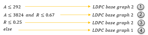
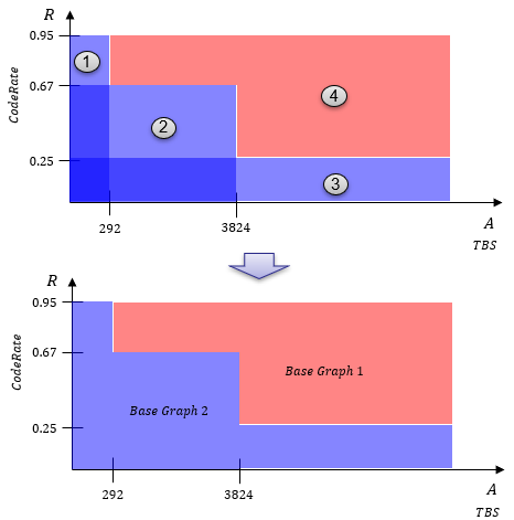
LDPC BaseGraph type is determined by Transport Size (A) and Code Rate(R) based on following criteria.
If I represent this as areas in coordinate, it would become as follows.
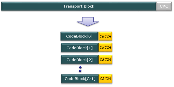
(3) Code block segmentation And Code Block CRC Attachment
This step is to ensure efficient and reliable data transmission by dividing large transport blocks into smaller segments and providing error detection capabilities at the code block level. We can think of this with a few different perspectives/steps summarized below.
Code Block Segmentation : If the size of a transport block is too large for efficient LDPC (Low-Density Parity-Check) coding, it is divided into smaller segments, called code blocks. The maximum size of a code block is defined by the 5G NR specifications. Segmentation is performed to ensure efficient channel coding and decoding while maintaining a reasonable complexity.Segmentation Criteria : The segmentation process is determined by comparing the transport block size with a specified maximum code block size. If the transport block size exceeds the maximum code block size, the transport block is divided into equal-sized code blocks (with the exception of the last code block, which may be smaller). If the transport block size is within the maximum code block size, no segmentation is performed.Code Block CRC Attachment : After segmentation, a CRC (Cyclic Redundancy Check) is calculated and attached to each code block individually. This 24-bit CRC allows for error detection at the receiver (UE) on a per-code-block basis.
The detailed procedures of this step can be summarized as follows.
i) Determine the max size of the code block (Kcb)
: The max size of the code block depends on LDPC base graph type as follows.
- For LDPC base graph type 1 : Kcb = 8448
- For LDPC base graph type 2 : Kcb = 3840
ii) Determine the number of Codeblocks
if B(Transport block size) < Kcb(Max Codeblock size)
L = 0
C (number of codeblocks) = 1
B' = B // this mean 'No Segmentation'.
else
L = 24
C = Ceiling(B/(Kcb - L))
B' = B + C * L
iii) Determine the number of bits in each code block
K'(the number of bits in each code block) = B'/C
iv) Determine Kb
For LDPC base graph type 1
Kb = 22
For LDPC base graph type 2
if B (Transport blocksize) > 640
Kb = 10
else if B (Transport blocksize) > 560
Kb = 9
else if B (Transport blocksize) > 192
Kb = 8
else
Kb = 6
v) find the minimum value of Z in all sets of lifting sizes in [38.212-Table 5.3.2-1: Sets of LDPC lifting size]
vi) denote Zc such that (Kb * Zc) >= K'
vii) set K = 22 Zc for LDPC base graph 1
K = 10 Zc for LDPC base graph 2
viii) perform segmentation and add CRC bits
s = 0 // s = bit position in B (transport block)
for r = 0 to C-1
for k = 0 to K'-L-1
crk = bs
s = s + 1
end for
if C > 1 // Do this if the number of the code block is more than 1
Calculate pr0,pr1,pr2,...,pr(L-1) using the sequence cr0,cr1,cr2,...,cr(K'-L-1) and g_CRC24B(D)
for k = K'-L to K'-1 // Append CRC bit
crk = pr(k+L-K')
end for
end if
for k = K' to K-1 // Insertion of filler bis
crk = < NULL >
end for
end for
The procedure can be summarized at high level as follows.
- Determine the maximum code block size (Kcb), which depends on the LDPC base graph type.
- Establish the number of code blocks (C), with segmentation occurring if the transport block size (B) exceeds Kcb.
- Calculate the bits in each code block (K'), dividing the modified transport block size (B') by the number of code blocks.
- Determine Kb, the size parameter for each code block, based on the transport block size and LDPC base graph type.
- Find the smallest lifting size (Z) from the specified set, ensuring Kb * Zc is greater than or equal to K'.
- Perform code block segmentation, append CRC bits for error checking, and add filler bits as necessary.
(4) Channel Coding
Detailed procedure of LDPC as described in 38.212 - 5.3.2 which is out of scope of this section (Beyond my knowledge as well :). Overall process can be summarized as below.
Parity Check Matrix : The LDPC codes are defined by a sparse parity-check matrix that represents the relationship between the data bits and the parity bits. 5G NR specifies two base graphs (Base Graph 1 and Base Graph 2) to construct the parity-check matrix, depending on the transport block size.Encoding :The LDPC encoding process takes the segmented code blocks (with attached CRC) as input and generates parity bits based on the chosen base graph and lifting factor. These parity bits are then appended to the original data bits, forming a codeword that is transmitted over the PUSCH.
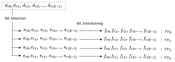
(5) Rate Matching
The Purpose of Rate matching is to adapts the output data rate of the channel encoder (LDPC) to match the available resources allocated for transmission in the time-frequency grid of the PUSCH. It can be describe in a few different steps as follows :
Bit Collection :: After LDPC coding, the encoded bits (data bits and parity bits) are collected in a circular buffer. The circular buffer is a temporary storage area with a fixed size that can hold bits in a circular manner, allowing for efficient bit selection.Bit Selection :: Depending on the allocated PDSCH resources, a specific number of bits are selected from the circular buffer. The selection process involves three main operations: bit interleaving, bit pruning, and bit puncturing.- Bit Interleaving: Rearranges the order of the bits to improve the robustness against burst errors during transmission.
- Bit Pruning: Removes any extra redundancy bits generated by the LDPC encoder
- Bit Puncturing: Discards some of the encoded bits (usually parity bits) if the number of encoded bits exceeds the allocated resources.
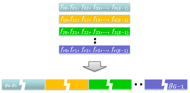
This is the step that combines the multiple code blocks resulting from the previous processing steps into a single data stream for transmission.
After rate matching, the processed code blocks are combined into a single data stream. The concatenation is performed in a specific order to ensure that the receiver (UE) can correctly separate and decode the individual code blocks. Typically, the code blocks are concatenated in the order they were segmented from the original transport block.
(7) Data and control multiplexing
Unlike PDSCH, PUSCH can carry UCI (control data) if it is configured. This step is to multiplexing the control data and user data. The entire process is long and complicated as described in 38.212 - 6.2.7.
- Bits for uplink shared channel (UL-SCH) and acknowledgments for Hybrid Automatic Repeat Request (HARQ-ACK) are denoted and sequenced according to the presence of CG-UCI when cg-UCI-Multiplexing is configured.
- Establishing sequences for Channel State Information (CSI) parts 1 and 2, if they are present.
- Identifying sequences for Uplink Control Channel Information (UCI) without HARQ-ACK.
- Multiplexing the data and control coded bits into a singular sequence, ensuring that the ordering reflects the priority of transmission.
- Calculating the OFDM symbol index for the scheduled PUSCH, accounting for all OFDM symbols used for DMRS
(8) Scrambling
Scrambling process is the step that introduces randomness to the transmitted data, ensuring uniform power distribution, interference management, data privacy, and accurate channel estimation. Scrambling and descrambling operations are performed at the transmitter and receiver, respectively, using the same cell-specific scrambling sequence. Scrambling introduces randomness to the transmitted data by applying a pseudo-random binary sequence (PRBS) to the data stream. This operation ensures that the transmitted signal has a uniform power distribution across different frequency and time resources.
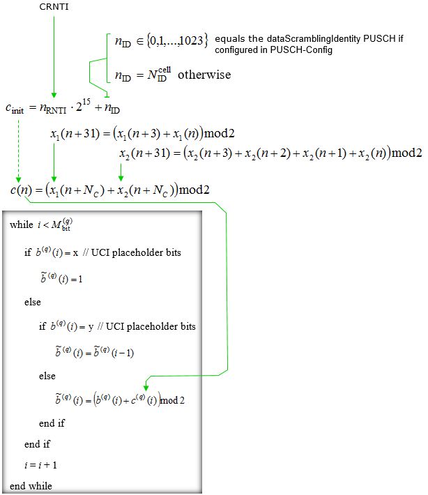
The high level summary of the above illustration is as follows :
- A scrambling identity n_ID is selected, which can be from a range if configured in PUSCH-Config, or based on the physical cell ID otherwise.
- The initial scrambling sequence c_init is computed using the RNTI, a power of 2, and the scrambling identity.
- Two pseudo-random sequences x1 and x2 are used to generate the scrambling sequence c(n).
- The binary sequence b'(i) is scrambled using the sequence c(i), with special handling for UCI placeholder bits.
- UCI placeholder bits are set to 1, and the scrambling process is continued for each bit of the binary sequence until the end of the block.
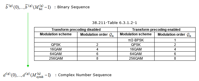
(9) Modulation
The modulation step is essential for converting the binary data stream into complex symbols suitable for wireless transmission. The choice of modulation scheme affects the data rate, spectral efficiency, and robustness against noise and interference. In 5G, 4 different modulation schemes are supported as of now.
- QPSK: QPSK modulates 2 bits per symbol, offering low data rates with high robustness against noise and interference.
- 16QAM: 16QAM modulates 4 bits per symbol, providing a balance between data rate and robustness.
- 64QAM: 64QAM modulates 6 bits per symbol, enabling higher data rates but with reduced robustness compared to QPSK and 16QAM.
- 256QAM: 256QAM modulates 8 bits per symbol, offering the highest data rates with the lowest robustness among the supported modulation schemes.
- pi/2 BPSK modulates 1 bits per symbol and used only when Transform precoding is enabled.
The choice of modulation scheme depends on factors such as channel conditions, link adaptation, and UE capabilities.
High level description of this process is :
The modulation process includes:
- A binary sequence denoted as b'(0), b'(1), ..., b'(Mbit - 1).
- Modulation schemes are selected based on the modulation order Qm.
- Schemes include pi/2 BPSK, QPSK, 16QAM, 64QAM, and 256QAM, with orders ranging from 1 to 8 as specified in 38.211-Table 6.3.1.2-1
- The binary sequence is converted into a complex number sequence d'(0), d'(1), ..., d'(Msymb - 1) for transmission.
The table in the image specifies the modulation order for each scheme, indicating the number of bits per symbol.
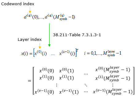
(10) Layer Mapping
Layer mapping is the step that distributes the modulated symbols across one or multiple layers for transmission using multiple antennas. It aims to improve the spectral efficiency, reliability, and capacity of the wireless communication system by utilizing advanced antenna techniques such as MIMO and beamforming. The mapping table is 38.211-Table 7.3.1.3-1 which is same as in PDSCH Layer Mapping.
(11) Transform Precoding
This is to convert the PUSCH data into the form of DFT-s-OFDM (a kind of SC-FDMA as in LTE PUSCH). This step is performed only transformprecoder in PUSCH-Config or msg3-transformPrecoding in RACH-ConfigCommon.
(12) Precoding
Mathemaically this step is pretty simple. Just mutiplying a matrix called Precoding matrix to the data from the previous step. But the problem is how to figure out the precoding matrix itself (i.e, how to determine the precoding matrix) is extremely complicated. Since this precoding matrix determination process is such a complicated, I had to create another page for the process. Refer to this page for the details of the process.
Just for the high level view, the precoding matrix is determined by two different method : codebook and non-codebook based.
In codebook based method, the matrix is determined by the information specified in DCI and some additional configurations in RRC message as follows.
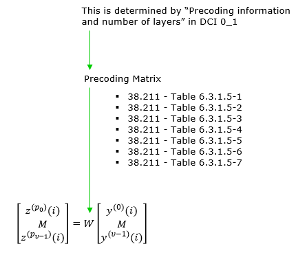
There are many difference types of tables to be applied for the precoding. Which table should be used for a specific case ? As shown below, depending on the number of layers, the number of antenna ports and on waveform type (transform precoding enabled or disabled), a specific precoding table is selected.
|
# of Layers |
# of Antenna Ports |
Transform Precoding |
Precoding Matrix (38.211) |
|
1 |
2 |
|
|
|
4 |
enabled |
||
|
disabled |
|||
|
2 |
2 |
disabled |
|
|
4 |
disabled |
||
|
3 |
4 |
disabled |
|
|
4 |
4 |
disabled |
In Non-codebook based method, the precoding matrix is determined by the measurement result of NZP-CSI-RS resource.
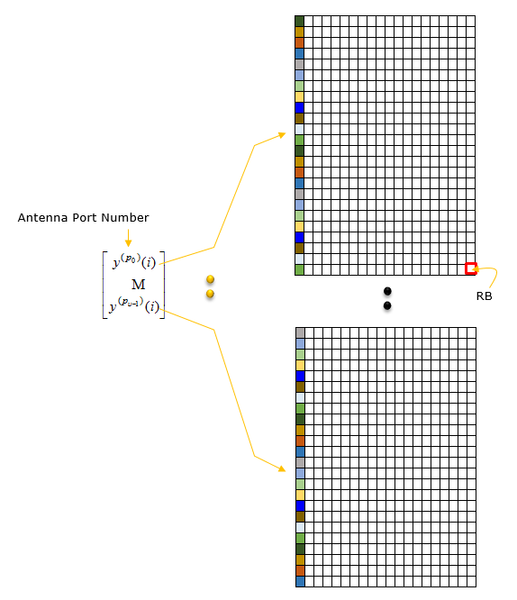
(13) Mapping to VRB
For each antenna step, a virtual resource grid is created. Within the resource grid, fill out each of the resource elements(RE) with PUSCH data from the RE at the lowest frequency to higher frequency. Once it reaches the RE at the highest frequency of the assigned PUSCH resource block, move to the RE at the lowest frequency of next OFDM symbol
Overall procedure goes as follows.
For each antenna port used for transmission of the PUSCH, a block of complex-valued symbols
z(p)(0), ..., z(p)(MAPsymb − 1)
is multiplied with the amplitude scaling factor βPUSCH to align with the transmit power specifications in TS 38.213 and mapped in sequence starting with
z(p)(0) to resource elements
(k', l)p,μ in the virtual resource blocks meeting the following criteria:
- The virtual resource blocks are assigned for the PUSCH transmission.
- The corresponding physical resource blocks are not used for transmission of associated DM-RS, PT-RS, or DM-RS intended for other co-scheduled UEs.
The mapping to resource elements allocated for PUSCH is in increasing order of the index k' over the assigned virtual resource blocks, where k'(subcarrier index) = 0 is the first subcarrier in the lowest-numbered virtual resource block, and then the index l(symbol index), with the starting position given by TS 38.214.
(14) Mapping from VRB to PRB
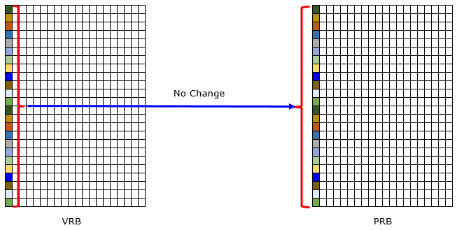
This step is the process that maps (converts) the virtual resource block(resource grid) into physical resource block(resource grid).
Two different types of mappings are supported in 5G as described below.
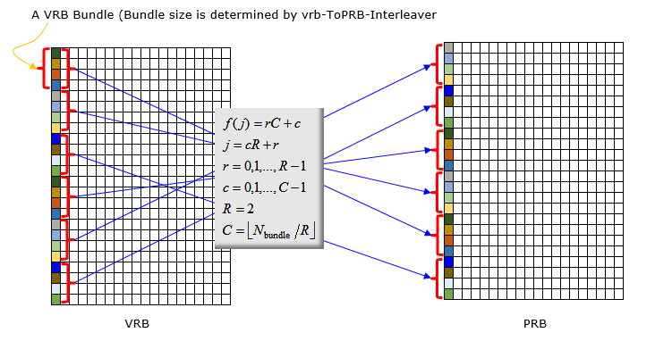
Non-Interleaved Mapping : In non-interleaved mapping, the modulated and precoded symbols are allocated to the physical resource blocks in a continuous and sequential manner. This strategy simplifies the mapping process but may result in reduced frequency diversity since adjacent symbols are transmitted on adjacent subcarriers.Advantages : Non-interleaved mapping is simple and straightforward, making it easy to implement and manage.Disadvantages : Due to the continuous allocation of symbols, non-interleaved mapping may be less resilient to frequency-selective fading and interference.Interleaved Mapping : In interleaved mapping, the modulated and precoded symbols are allocated to the physical resource blocks in a non-sequential and dispersed manner. This strategy increases frequency diversity by spreading the symbols across the available resources, improving resilience against frequency-selective fading and interference.Advantages : Interleaved mapping provides better frequency diversity and is more robust against frequency-selective fading and interference, which can improve the overall system performance.Disadvantages : The increased complexity of interleaved mapping can make it more challenging to implement and manage compared to non-interleaved mapping.
< Non-Interleaved >
This is illustration of Non-Interleaved mapping from VRB to PRB
< Interleaved >
This is illustration of Interleaved mapping from VRB to PRB
RRC Parameters
38.331 15.3 (2018-10)
PUSCH-Config ::= SEQUENCE {
dataScramblingIdentityPUSCH INTEGER (0..1023) OPTIONAL,
txConfig ENUMERATED {codebook, nonCodebook}
dmrs-UplinkForPUSCH-MappingTypeA SetupRelease { DMRS-UplinkConfig }
dmrs-UplinkForPUSCH-MappingTypeB SetupRelease { DMRS-UplinkConfig }
pusch-PowerControl PUSCH-PowerControl
frequencyHopping ENUMERATED {intraSlot, interSlot}
frequencyHoppingOffsetLists SEQUENCE (SIZE (1..4)) OF
INTEGER (1.. maxNrofPhysicalResourceBlocks-1)
resourceAllocation ENUMERATED { resourceAllocationType0,
resourceAllocationType1,
dynamicSwitch},
pusch-TimeDomainAllocationList SetupRelease {
PUSCH-TimeDomainResourceAllocationList
}
pusch-AggregationFactor ENUMERATED { n2, n4, n8 }
mcs-Table ENUMERATED {qam256, qam64LowSE}
mcs-TableTransformPrecoder ENUMERATED {qam256, qam64LowSE}
transformPrecoder ENUMERATED {enabled, disabled}
codebookSubset ENUMERATED {fullyAndPartialAndNonCoherent,
partialAndNonCoherent,
nonCoherent}
maxRank INTEGER (1..4)
rbg-Size ENUMERATED { config2}
uci-OnPUSCH SetupRelease { UCI-OnPUSCH }
tp-pi2BPSK ENUMERATED {enabled}
...
}
UCI-OnPUSCH ::= SEQUENCE {
betaOffsets CHOICE {
dynamic SEQUENCE (SIZE (4)) OF BetaOffsets,
semiStatic BetaOffsets
} OPTIONAL, -- Need M
scaling ENUMERATED { f0p5, f0p65, f0p8, f1 }
}
|
pusch-AllocationList |
|
|
row 0 |
PUSCH-TimeDomainResourceAllocation ::= SEQUENCE { k2 INTEGER (0..7) mappingType ENUMERATED {typeA, typeB}, startSymbolAndLength BIT STRING (SIZE (7)) // SLIV } |
|
row 1 |
PUSCH-TimeDomainResourceAllocation ::= SEQUENCE { k2 INTEGER (0..7) mappingType ENUMERATED {typeA, typeB}, startSymbolAndLength BIT STRING (SIZE (7)) // SLIV } |
|
... |
... |
|
row N |
PUSCH-TimeDomainResourceAllocation ::= SEQUENCE { k2 INTEGER (0..7) mappingType ENUMERATED {typeA, typeB}, startSymbolAndLength BIT STRING (SIZE (7)) // SLIV } |
PUSCH-ConfigCommon ::= SEQUENCE {
groupHoppingEnabledTransformPrecoding ENUMERATED {enabled} OPTIONAL, -- Need R
pusch-AllocationList SEQUENCE (SIZE(1..maxNrofUL-Allocations))
OF PUSCH-TimeDomainResourceAllocation OPTIONAL, -- Need R
msg3-DeltaPreamble INTEGER (-1..6) OPTIONAL, -- Need R
p0-NominalWithGrant INTEGER (-202..24) OPTIONAL, -- Need R
...
}
Reference
[1]