|
SDR(Software Defined Radio) |
||
|
RTL2832/Matlab Example
Example 1 : Basic Capture and Visualize
One of the most tricky part of learning any new technology or new tool is to figure out the very first/the most basic connection method or command. When I was learning about electric circuit (a small embedded system) was to figure out how to turn on and off the small LED on the board. Everytime when I was trying to learn new computer language, the first thing I was trying to figure out is how to create a program to print out "Hello World". Then what is the Hello World part of MatLab RTL ? It would be to get Matlab connected to the hardware and read a bunch of data (I/Q data) captured by the hardware. This is done by the simple two steps as below. obj_hardwareHandle = comm.SDRRTLReceiver(...) raw_data = step(obj_hardwareHandle); The first line is to define which hardware it want to connect and what kind of configuration you want to apply to the hardware. This line itself does not do anything to the hardware, it is just definition of the configuration. The real work of communicating and controlling hardware is done by the second line. The step(obj_hardwareHandle) connect to the hardware and let it capture the signal as defined in the first line and read the captured data and store it to a variable called 'raw_data'. This is all you need to know of Matlab RTL. Once you have the data stored in a variable (e.g, raw_data as in this tutorial), all the remaining procedure is up to you and knowledge about generic Matlab function and radio technology.
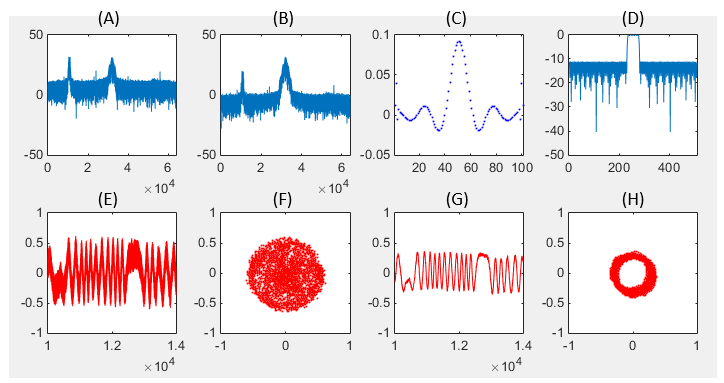
The outcome of the simple tutorial that I will show in this post is as show below.
Following is short descriptions on each of the plots shown above. (A) : Frequency domain data from the captured data (the result of fft of raw_data) (E) : Real values of raw data (I data) captured by the hardware. (real part of raw_data). (F) : Real and Imaginary data of raw_data plotted in Cartesian coordinate (I/Q plane plot, Constellation) (C) : Time domain representation of a digitial filter (D) : Frequency domain representation of the digital filter. (B) : The result of applying the digital filter (C,D) to data (A) (G) : The result of applying the digital filter (C,D) to data (E) (H) : The result of applying the digital filter (C,D) to data (F)
Following is the matlab source code that I used to get the result shown above. The green part is the critical part for Matlab to capture the data from the hardware and all the remaining part is just generic Matlab fuctions that you might already be familiar with. clear all;
RTL_USB_ID = '0'; RTL_USB_CarrierFrequency = 91.5e6; RTL_USB_Gain = 30; RTL_USB_SamplingFrequency = 2.4e6; RTL_USB_ppm = 0; RTL_USB_FrameLength = 256*250; RTL_USB_DataType = 'single';
Handle_RTL_USB = comm.SDRRTLReceiver(... RTL_USB_ID,... 'CenterFrequency', RTL_USB_CarrierFrequency,... 'EnableTunerAGC', true,... 'SampleRate', RTL_USB_SamplingFrequency, ... 'SamplesPerFrame', RTL_USB_FrameLength,... 'OutputDataType', RTL_USB_DataType,... 'FrequencyCorrection', RTL_USB_ppm);
raw_data = step(Handle_RTL_USB);
a = 1; b = firpm(100,[0,10e3,12e3,(240e3/2)]/(240e3/2), [1 1 0 0], [1 1], 40); y = filter(b,a,raw_data);
block = 10000:14000;
subplot(2,4,1); plot(10*log10(abs(fftshift(fft(raw_data)))));xlim([0 length(raw_data)]); ylim([-50 50]);
subplot(2,4,2); plot(10*log10(abs(fftshift(fft(y)))));xlim([0 length(y)]); ylim([-50 50]);
subplot(2,4,3); plot(b,'bo','MarkerFaceColor',[0 0 1],'MarkerSize',1); xlim([1 length(b)]);
subplot(2,4,4); plot(10*log10(abs(fftshift(fft(b,512))))); xlim([0 512]); ylim([-50 0]);
subplot(2,4,5); plot(block,real(raw_data(block)),'r-'); xlim([block(1) block(end)]); ylim([-1 1]);
subplot(2,4,6); plot(real(raw_data(block)),imag(raw_data(block)),'ro','MarkerFaceColor',[0 0 1],'MarkerSize',1); axis([-1 1 -1 1]);
subplot(2,4,7); plot(block,real(y(block)),'r-'); xlim([block(1) block(end)]); ylim([-1 1]);
subplot(2,4,8); plot(real(y(block)),imag(y(block)),'ro','MarkerFaceColor',[0 0 1],'MarkerSize',1); axis([-1 1 -1 1]);
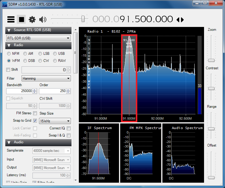
My next trials was to write a Matlab code to do similar things as SDRsharp. I wanted to set the frequency as shown below (You would need to set other frequencies depending on where you are) and listen the Radio from Matlab. However, it was not as easy as I have thought. I spent a couple of days to figure out proper parameters values and routines that make this possible. The Reference [1] helped a lot, but I needed to put extra time and effort to find parameters values for this Radio and to create some additional filters for clearer sound. Even with all the efforts, the result was not as good as SDRsharp but at least I could listen and understand the broadcast with a little bit of noise.
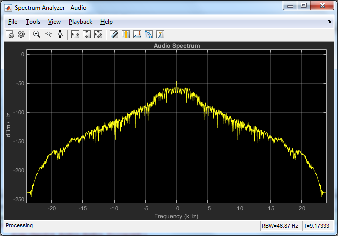
Following is a snapshot of the real time audio spectrum and you would be able to listen the radio while this spectrum gets updated.
Following is my code to listen to the broadcase.
% Define Parameters for RTL Device. % The tricky part for me was to find proper value for RTL_USB_FrameLength. If it is too short, I could % hear a kind of knocking sound. If it is too long, you would see too slow update for audio spectrum. % In addition, Maximum frame length is just a little bit ver 300,000bits and this number should be % a integer multiples of Decimation Factors.
RTL_USB_ID = '0'; RTL_USB_CarrierFrequency = 91.5e6; RTL_USB_Gain = 30; RTL_USB_SamplingFrequency = 2.4e6; RTL_USB_ppm = 0; RTL_USB_FrameLength = 256*20*50; RTL_USB_DataType = 'single'; AudioFrequency = 48e3; PlayTime = 20;
RTL_USB_FrameTime = RTL_USB_FrameLength/RTL_USB_SamplingFrequency;
% Define a Handle to SDR RTL Device % A parameter you need to set carefully would be 'EnableTunerAGC'. In my example, % I set it as 'true' meaning that the Gain is set automatically by the RTL hardware. % you can set a specific Gain value if you like, but in that case the signal level % coming into RTL antenna should be good and should not fluctuating too much. Handle_RTL_USB = comm.SDRRTLReceiver(... RTL_USB_ID,... 'CenterFrequency', RTL_USB_CarrierFrequency,... 'EnableTunerAGC', true,... 'SampleRate', RTL_USB_SamplingFrequency, ... 'SamplesPerFrame', RTL_USB_FrameLength,... 'OutputDataType', RTL_USB_DataType,... 'FrequencyCorrection', RTL_USB_ppm);
% Define a Handle to an Audio Player Handle_Audio = dsp.AudioPlayer(AudioFrequency);
% Define a Handle to Spectrum Analyzer Handle_AudioSpectrum = dsp.SpectrumAnalyzer(... 'Name', 'Spectrum Analyzer - Audio',... 'Title', 'Audio Spectrum',... 'SpectrumType', 'Power density',... 'FrequencySpan', 'Full',... 'SampleRate', AudioFrequency);
% design a filter for the captured signal (raw data) % With the current Antenna and location, the demodulated audio came in with a lot of noise % I tried to filter out the noise at Audio stage only, but the result was not satisfactory. % So I designed a filter to reduce the noise from the raw data. % You may play with this filter parameters for your setup fir_a = 1; fir_b = firpm(100,[0,15e3,20e3,(240e3/2)]/(240e3/2), [1 1 0 0], [1 1], 40);
% design a filter for audio signal (demodulated data) % This is the filter to reduce the noise at Audio stage. % You may play with this filter parameters for your setup [iir_b,iir_a] = butter(4,(2500)/(AudioFrequency/2));
run_time = 0;
while run_time < PlayTime
% Capture I/Q Data from Hardware and Store it to RTL_USB_RawData RTL_USB_RawData = step(Handle_RTL_USB);
% apply the filters to the captured data RTL_USB_Filtered = filter(fir_b,fir_a,RTL_USB_RawData);
% Calculate the Phase Differences RTL_USB_Filtered_Delay_1 = circshift(RTL_USB_Filtered,1); RTL_USB_Filtered_Conjugate = conj(RTL_USB_Filtered); RTL_USB_Filtered_PhaseDifference = ... angle(RTL_USB_Filtered_Conjugate .* RTL_USB_Filtered_Delay_1);
% decimate the data by the factor of 50. % This convert 2.4Mhz sample to 48 Khz (2.4 Mhz/50) sample RTL_USB_Filtered_PhaseDifference_Decimated = ... decimate(double(RTL_USB_Filtered_PhaseDifference),50,8);
% Apply the iir filter to the audio data Audio_Filtered = ... filter(iir_b,iir_a,RTL_USB_Filtered_PhaseDifference_Decimated);
% Plot the audio data on Spectrum step(Handle_AudioSpectrum, Audio_Filtered);
% Play the Audio data step(Handle_Audio,Audio_Filtered);
run_time = run_time + RTL_USB_FrameTime;
end
Example 3 : Capturing RKE Signal
One of the difficulties I had with playing with RTL device was it is Reciever only hardware.. it does not have any transmitter functionality. The easiest function you can play with would be Radio Broadcast, but the motivation would not last long. Next stage would be to try with signals other than Radio Broadcast like GPS and others, but in those case you may need speciall antenna being installed out side of home or office. I was looking for some other signal that I can play with without any extra investment. Then.. one day my car key caught my attention and I decided to try using my Car key as a signal generator. The result was very satisfactory and this example is about playing with my Car Key. Since I am in North America, the frequency of the RKE is expected to be 315 Mhz, but I wanted to check the exact frequency first. Each of the Key may have a little bit of variations of all. So I confirmed on the frequency with SDRSharp as described in SDRSharp tutorial : Capturing RKE(Remote Key Entry) Signal.
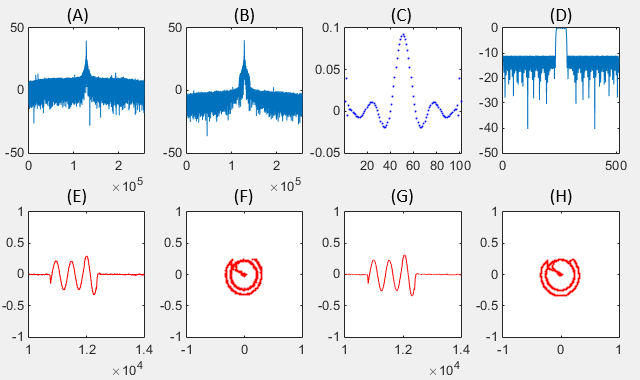
Next trial was to use the Matlab code from Example 1 without any modification just to capture the signal and display it. The purpose of this part is just to capture the I/Q Data. So the meaningful part would be (A),(E),(F) in this example.
Following is short descriptions on each of the plots shown above. (A) : Frequency domain data from the captured data (the result of fft of raw_data) (E) : Real values of raw data (I data) captured by the hardware. (real part of raw_data). (F) : Real and Imaginary data of raw_data plotted in Cartesian coordinate (I/Q plane plot, Constellation) (C) : Time domain representation of a digitial filter (D) : Frequency domain representation of the digital filter. (B) : The result of applying the digital filter (C,D) to data (A) (G) : The result of applying the digital filter (C,D) to data (E) (H) : The result of applying the digital filter (C,D) to data (F)
Following is the source code that produced the plot shown above. clear all;
% Define Parameters for RTL Device.
RTL_USB_ID = '0'; RTL_USB_CarrierFrequency = 314.4e6; RTL_USB_Gain = 30; RTL_USB_SamplingFrequency = 2.4e6; RTL_USB_ppm = 0; RTL_USB_FrameLength = 256*20*50; RTL_USB_DataType = 'single';
% Define a Handle to SDR RTL Device % A parameter you need to set carefully would be 'EnableTunerAGC'. In my example, % I set it as 'true' meaning that the Gain is set automatically by the RTL hardware. % you can set a specific Gain value if you like, but in that case the signal level % coming into RTL antenna should be good and should not fluctuating too much.
Handle_RTL_USB = comm.SDRRTLReceiver(... RTL_USB_ID,... 'CenterFrequency', RTL_USB_CarrierFrequency,... 'EnableTunerAGC', true,... 'SampleRate', RTL_USB_SamplingFrequency, ... 'SamplesPerFrame', RTL_USB_FrameLength,... 'OutputDataType', RTL_USB_DataType,... 'FrequencyCorrection', RTL_USB_ppm);
% Following line activate hardware and capture the I/Q data and store it in the variable raw_data
raw_data = step(Handle_RTL_USB);
% Following is a digital filter to remove the noise from the captured signal. But the parameters for the filter is % not specially optimized for the RKE. I just used the same parameters that I used for FM demodulation. % You may try with different parameters optimized for RKE if you want. % It would be good for you to understand digital filter parameters. a = 1; b = firpm(100,[0,10e3,12e3,(240e3/2)]/(240e3/2), [1 1 0 0], [1 1], 40); y = filter(b,a,raw_data);
% this is to specify the range of the data to cut out from the captured data (raw_data). Since I captured % pretty many samples, it would take too long time to plot if you try to plot it all.
block = 10000:14000;
% Followings are for producing those plots shown above.
subplot(2,4,1); plot(10*log10(abs(fftshift(fft(raw_data)))));xlim([0 length(raw_data)]); ylim([-50 50]);
subplot(2,4,2); plot(10*log10(abs(fftshift(fft(y)))));xlim([0 length(y)]); ylim([-50 50]);
subplot(2,4,3); plot(b,'bo','MarkerFaceColor',[0 0 1],'MarkerSize',1); xlim([1 length(b)]);
subplot(2,4,4); plot(10*log10(abs(fftshift(fft(b,512))))); xlim([0 512]); ylim([-50 0]);
subplot(2,4,5); plot(block,real(raw_data(block)),'r-'); xlim([block(1) block(end)]); ylim([-1 1]);
subplot(2,4,6); plot(real(raw_data(block)),imag(raw_data(block)),'ro','MarkerFaceColor',[0 0 1],'MarkerSize',1); axis([-1 1 -1 1]);
subplot(2,4,7); plot(block,real(y(block)),'r-'); xlim([block(1) block(end)]); ylim([-1 1]);
subplot(2,4,8); plot(real(y(block)),imag(y(block)),'ro','MarkerFaceColor',[0 0 1],'MarkerSize',1); axis([-1 1 -1 1]);
% Save the 'raw_data' into a csv file. This saved file will be used for analysis in next step. dlmwrite('rke_315_01.dat',raw_data,'newline','pc');
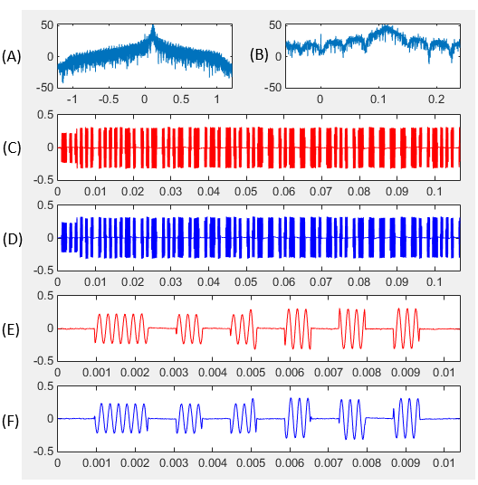
Next step was to analyze the data captured above in more detail. Followings are the result of the analysis (very simple analysis) for the data saved in the csv file.
Following is short descriptions on each of the plots shown above. (A) : Frequency domain data from the captured data (the result of fft of the decimated raw_data) (B) : The same data as shown in (A) but showing the only portions around the carrier frequency. (C) : Real Part of raw_data (I data of the decimated raw_data). (D) : Imaginary Part of raw_data (Q data of the decimated raw_data). (E) : Same data as (C), but showing only short blocks (defined by chunk_range in the code) (F) : Same data as (D), but showing only short blocks (defined by chunk_range in the code)
Following is the source code that produced the result as shown above. clear all;
% following is to read the data from the data file. You see I transposed the read data, but no special % methematical reason for the transpose. It is just to match the dimension (vector dimension) with % other variables like 't' and 'f' that will be created later.
raw_data = csvread('rke_315_01.dat'); raw_data = raw_data';
% Following is to decimate (undersample) the capture data. Since the number of samples that I captured % is pretty big and the signal bandwidth is much narrower than the sampling bandwidth. I decided to % undersample the data to increase the speed of next level processing (like plotting)
decimation_factor = 25; decimated_data = decimate(double(raw_data),decimation_factor,8);
% Following is to create tick marks for time domain and frequency domain. t = linspace(0,length(decimated_data)-1,length(decimated_data)) ./ (2.4e6/decimation_factor); f = linspace(0,2.4e6,length(t))/1e6; f = f - 0.5*max(f);
% Following is the cut out a specific portions of data from decimated_data to magnify the plot % in horizontal axis. chunk_range = 1:1000;
% Followings are plotting routine that generates the plots shown above. subplot(5,2,1); freq_dB = 20*log10(abs(fftshift(fft(decimated_data)))); plot(f,freq_dB); xlim([f(1) f(end)]); ylim([-50 max(freq_dB)]);
subplot(5,2,2); freq_dB = 20*log10(abs(fftshift(fft(decimated_data)))); plot(f,freq_dB); xlim([0.05*min(f) 0.2*max(f)]); ylim([-50 max(freq_dB)])
subplot(5,2,[3 4]); plot(t,real(decimated_data),'r-'); xlim([t(1) t(end)]);
subplot(5,2,[5 6]); plot(t,imag(decimated_data),'b-'); xlim([t(1) t(end)]);
subplot(5,2,[7 8]); plot(t(chunk_range),real(decimated_data(chunk_range)),'r-'); xlim([t(chunk_range(1)) t(chunk_range(end))]);
subplot(5,2,[9 10]); plot(t(chunk_range),imag(decimated_data(chunk_range)),'b-'); xlim([t(chunk_range(1)) t(chunk_range(end))]);
Reference :
[1] Software_Defined_Radio_using_MATLAB_Simulink_and_the_RTL-SDR
|
||