Predistortion

Predistortion is a technique which can compensate the influence of distortion created by an amplifier. As you know, Amplifier is a device that maginfies the input signal and output a larger signal. Ideal amplifier should amplifies the signal in the same degree whether the input signal level is low or high. However, in reality most of amplifier amplifies a little different degree depending on the input level. This different level of amplification depending on signal level would result in the distortion of the signal and this distortion would cause various unwanted outcomes. One of the biggest problem is that the distortion would cause large degree of power leakage out of the signal bandwidth.

Would there be any way to minimize the effect of distortion ? One possible idea is that to distort the signal in the exactly opposite way that the amplifier will distort before the signal goes into the amplifier. This technique is called 'Predistortion' meaning 'Distortion Before Amplifier'.

In practice the correction runs in the digital baseband, before the DAC, so it is usually called digital predistortion or DPD. Two effects need correcting. AM/AM distortion is a gain that changes with the input amplitude. AM/PM distortion is a phase shift that changes with the input amplitude. This page starts with the gain effect in a simple time domain model. Then it looks at the spectrum, and at the two ways to find the predistortion function.

Why does the amplifier distort a large signal ?

Let's start with one amplifier and two input signals of different size. Why does the same amplifier leave a small signal clean and distort a large one? The answer is in the shape of the transfer function, not in the value of the gain.

Let's assume that you have an amplifier and the transfer function (operating function) of the amplifier looks like the plot at the center of the following illustration. With just a glimpse, you would notice the transfer function is not linear, meaning the degree of amplification varies depending on the level of the input signal.

Now let's look at the figure at upper track. A signal (green plot) with relatively low level goes into the amplifier (top-left). After going through the amplifier, you would have the output signal shown in blue color. If you compare the input signal and output signal, you would notice the shape of the signal is almost same. It means that the input signal is not distorted by the amplification. (I intentionally used the transfer function with gain of 1 for easy comparison of the two signal).

Now look at the graph in lower track. You see a little wide range of signal (green plot) goes into the amplifier. In this case, you will see some difference between the shape of input signal (green color) and output signal (blue color) especially upper range of the signal. It means that the signal get distorted by the amplifier.

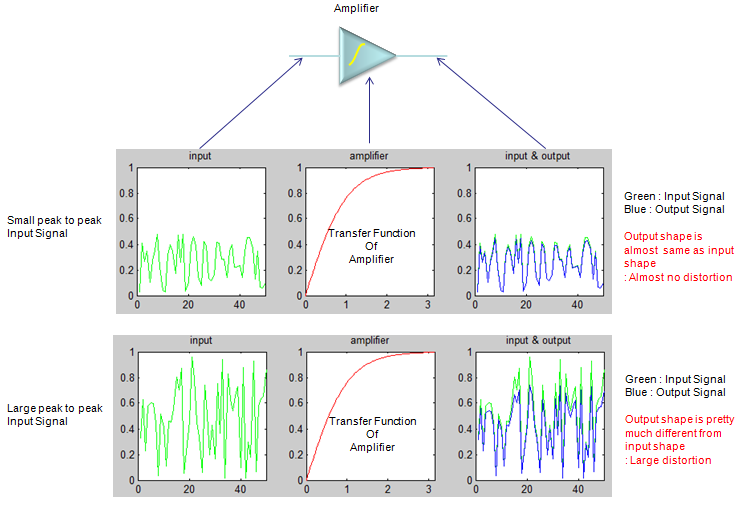
Amplifier transfer function applied to a small and a large input signal, with input, amplifier curve and input and output plots for each

One amplifier, two input levels. The small signal stays on the straight part of the curve, and the large signal reaches the flat part.

The amplifier symbol at the top points to the three plots of each row: input, amplifier, and input & output.
The amplifier plot draws the transfer function in red. It rises almost straight from 0 and flattens towards 1 above an input of about 2.
In the upper row, labelled Small peak to peak Input Signal, the green input stays below about 0.5. The blue output nearly covers it, and the red note reads Almost no distortion.
In the lower row, labelled Large peak to peak Input Signal, the input spans about 0 to 1. The blue output stays visibly below the green input near the top, and the note reads Large distortion.

The numbers behind the plots are easy to check. The code models the amplifier as tanh(x), whose slope at 0 is 1. So a small input comes out almost unchanged. At an input of 1, tanh gives 0.76, which is about 2.4 dB of gain compression. The peaks of the large signal are squeezed, but its low values are not. This uneven gain is the distortion.

If you want to play with this process a little bit further, try with the following Matlab/Octave code. You can play with inputmin and inputmax value as you like to change the input signal level and see how the output signal changes.

gain = 1.0;

x = 0:pi/100.0:pi;

y_amp = gain * tanh(x);

inputmin = 0.0;

inputmax = 1.0;

inputsize = 50;

input = inputmin + (inputmax-inputmin) * rand(1,inputsize);

output = gain * tanh(input);

subplot(1,3,1);plot(input,'g-');title('input');xlim([0 length(input)]);ylim([0 1]);

subplot(1,3,2);plot(x,y_amp,'r-');title('amplifier');xlim([0 max(x)]);ylim([0 1]);

subplot(1,3,3);plot(input,'g-');hold on;plot(output,'b-');hold off;

title('input & output');xlim([0 length(input)]);ylim([0 1]);

The distortion depends on the signal level : the same amplifier is nearly linear for small inputs and compresses large ones.
Compression hits the peaks first : at an input of 1 the tanh model gives 0.76, about 2.4 dB below a linear gain.
A large peak to peak signal suffers most : its peaks reach the flat part of the curve.

How does predistortion cancel the amplifier distortion ?

The distortion comes from a known curve, so a second curve can undo it. Predistortion places that second curve in front of the amplifier. Its transfer function is the inverse of the amplifier curve, so the two curves in series give a straight line.

Now the question is "Is there any way to minimize or remove the distortion effect ?".

Presenter pointing at a board with the question How can we reduce the distortion for large peak to peak signal

The question for this section: how to reduce the distortion of a signal with a large peak to peak range.

One idea is to add another block right in front of the amplifier as shown below. Let's assume that the transfer function of the predistortion block is as shown below. Let's see how the signal changes after it went through the distortion block. You would notice pretty big difference between the output signal (blue color) and input signal (green color) meaning that it is 'distorted'. But this distortion is 'wanted/intended' distortion.

And then this distorted signal (not the original signal) goes through the amplifier. Now see how the signal coming out of the amplifier looks like. You will see that the shape of the output signal is almost same as the input signal.

This shows that the intentional distortion created by the predistortion block has removed the effect of distortion by the amplifier.

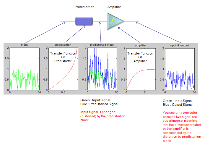
Predistortion block followed by an amplifier, with plots of input, predistortion curve, predistorted input, amplifier curve and input and output

Predistortion and amplifier in series. The blue output lies on the green input, so the two distortions cancel.

The block diagram at the top puts Predistortion before Amplifier. Arrows link each block and each signal point to one of the five plots below.
The predistortion plot draws a red curve that bends upward, the opposite of the amplifier curve. It reaches 2, the top of the axis, at an input just under 1.
The predistorted Input plot shows the blue predistorted signal above the green input. The largest blue peaks run past the top of the axis.
The input & output plot shows a single blue trace. The red note explains that the green input is hidden under the blue output.

gain = 1.0;

x = 0:pi/100.0:pi;

y_amp = gain * tanh(x);

x_pre = 0:1/100.0:0.99;

y_pre = gain * atanh(x_pre);

inputmin = 0.0;

inputmax = 1.0;

inputsize = 50;

input = inputmin + (inputmax-inputmin) * rand(1,inputsize);

predistortedInput = atanh(input);

output = gain * tanh(predistortedInput);

subplot(1,5,1);plot(input,'g-');title('input');xlim([0 length(input)]);ylim([0 2]);

subplot(1,5,2);plot(x_pre,y_pre,'r-');title('predistortion');xlim([0 max(x_pre)]);ylim([0 2]);

subplot(1,5,3);plot(input,'g-');hold on;plot(predistortedInput,'b-');hold off;

title('predistorted Input');xlim([0 length(input)]);ylim([0 2]);

subplot(1,5,4);plot(x,y_amp,'r-');title('amplifier');xlim([0 max(x)]);ylim([0 2]);

subplot(1,5,5);plot(input,'g-');hold on;plot(output,'b-');hold off;

title('input & output');xlim([0 length(input)]);ylim([0 2]);

The code uses atanh as the predistortion function, because atanh is the exact inverse of tanh. So output = tanh(atanh(input)) returns the input itself, and that is why only one trace is visible. Now look at the predistorted Input plot again. As the input approaches 1, atanh grows without limit. For example, atanh(0.99) is about 2.65, so the blue peaks leave the axis.

This shows the real limit of predistortion. The tanh amplifier never outputs more than 1, whatever its input. So predistortion can straighten the curve only below the saturation level. A peak that needs an output above saturation cannot be restored. For this reason, a transmitter usually runs crest factor reduction together with DPD. Crest factor reduction keeps the peaks inside the range that the predistorter can correct.

The predistorter is the inverse of the amplifier : in the code, atanh in front of tanh gives a straight line.
The predistorter must overdrive the peaks : its output grows without limit as the amplifier output approaches saturation.
Saturation cannot be corrected : predistortion linearises only the range below the maximum output of the amplifier.

What does predistortion change in the spectrum ?

The time domain plots show the shape of the signal. But the neighbouring channels see the spectrum, and there the distortion appears as power outside the assigned channel. Let's connect the two views before looking at measured spectra.

A nonlinear curve can be written as a polynomial. Its odd terms, such as x³ and x⁵, mix the frequencies inside the signal with each other. For a signal of bandwidth B, the third order products cover about 3B and the fifth order products about 5B, centred on the carrier. This spreading is called spectral regrowth. ACLR measures how much of it falls into the adjacent channel.

What I explained above is mostly based with time domain characteristics, but in reality handling amplifiers you would characterize them more in frequency domain. If you compare the frequency response of unlinearized (without predistortion) and linearized (with predistortion), it can be illustrated as below. As you see, the most critical issue caused by operating in nonlinear region without predistortion is high ACLR/ACPR as shown in gray traces as shown below. With proper predistortion, you can remove those high ACLR/ACPR to make it like black trace shown below.

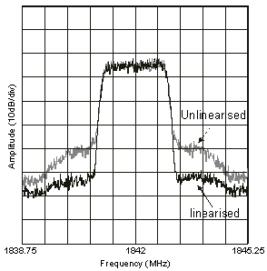
Base station amplifier output spectrum around 1842 MHz, unlinearised trace in grey and linearised trace in black

Output spectrum with and without linearisation. Outside the carrier, the linearised shoulders sit about one division, 10 dB, lower.

Image from the article Linear Power Amplifiers for 3G (W-CDMA) Base Stations

The horizontal axis runs from 1838.75 MHz to 1845.25 MHz, with the carrier at 1842 MHz. The vertical axis is Amplitude at 10 dB/div.
The grey trace is labelled Unlinearised. Its shoulders fall slowly from the carrier edges towards the sides of the plot.
The black trace is labelled linearised. Its shoulders drop almost straight to the floor on both sides of the carrier.
Inside the carrier the two traces overlap. The benefit of linearisation is entirely outside the channel.

Following is another example of showing the effect of (digital) Predistortion from the datasheet of AD9375(Analog Device). Red plot shows the case Without Predistortion and the Blue plot shows With Predistortion.

AD9375 datasheet Figure 232 and Figure 233, LTE output spectrum with DPD in blue and without DPD in red, for 20 MHz and 40 MHz signals

AD9375 datasheet Figure 232 and Figure 233. With DPD, the power next to the carrier drops by about 20 dB for both signals.

Figure 232 on the left is a 20 MHz LTE signal at 2600 MHz, with the carrier near +9 dBm. Without DPD, the red skirt reaches about -20 dBm at the carrier edges. With DPD, the blue trace sits near -40 dBm there.
The red skirt changes slope near 2570 MHz and 2630 MHz. That span is 60 MHz, three times the signal bandwidth, which matches the extent of the third order products.
Figure 233 on the right is a 40 MHz LTE output with the carrier near 0 dBm and a narrow notch at 2600 MHz. The shoulders fall from about -30 dBm without DPD to below -45 dBm with DPD.
Far from the carrier, the red and blue traces come together. There the nonlinearity no longer sets the level.

Distortion in time is regrowth in frequency : odd order products spread a signal of bandwidth B to about 3B and 5B.
ACLR is the number that captures it : it compares the power in the adjacent channel with the power in the assigned channel.
DPD gains about 20 dB next to the carrier : in the AD9375 plots, for both the 20 MHz and the 40 MHz LTE signal.

How is the predistortion function found ?

Now the most important question would be "How can I know the degree of predistortion for a specific amplifier ?". More technically speaking, how can I figure out the transfer function of predistortion block ?

Theoretical answer is very simple. If you know the transfer function of the amplifier, you can get the transfer function of the predistortion block just by taking the inverse function of the transfer function.

As you know, in reality nothing goes as easy as you say. For further details of predistortion (especially implementation of predistortion), please refer to other materials. you can google out a lot of articles/posts. I think this is enough for explaining the concept of the predistortion.

The inverse is harder to get than it sounds, for three reasons. The first is AM/PM distortion, so the predistorter must correct the phase as well as the gain. The second is memory effects. With a wideband signal, the output depends on recent input samples as well as the present one, so a single curve no longer describes the amplifier. For this reason, wideband DPD often models the amplifier with a memory polynomial. The third is drift. The amplifier curve changes with temperature, supply voltage, carrier frequency and ageing.

Basically there are two method of define the degree of predistortion, open-loop method and closed-loop method. (This is also a kind of control system, so it would be either open-loop or closed-loop).

Open-loop method - lookup table

In open-loop method as shown below, we use a kind of predefined lookup table to specify the degree of predistortion. This method would be simple to implement but the question is what would be the best lookup table and how can we create the table.

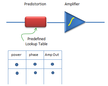
Open-loop predistortion with a predefined lookup table of power, phase and amplifier output feeding the predistortion block

Open-loop predistortion. A predefined lookup table sets the correction, and nothing measures the result.

The red Predistortion block sits before the blue Amplifier on one signal line. No path returns from the output.
A green arrow ties the predistortion block to the Predefined Lookup Table below it.
The table has three columns: power, phase and Amp Out. The dots stand for the entries, one row per power level.

The table is filled once, from measurements of the amplifier, for example in the factory. That is the weak point of this method. When the temperature or the carrier frequency changes, the amplifier curve changes too, but the table does not.

Closed-loop method - feedback

In closed loop method as illustrated below, the output of the amplifier feedback to the predistortion block and the block adaptively figure out the proper predistortion parameter based on the feedback. The advantage would be that this method would dynamically adjust the value but implementation of adaptive algorithm would be difficult.

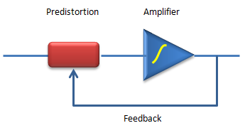
Closed-loop predistortion with a feedback path from the amplifier output back to the predistortion block

Closed-loop predistortion. The amplifier output returns to the predistortion block through the Feedback path.

The Predistortion and Amplifier blocks sit on one signal line, as in the open-loop drawing.
A line labelled Feedback leaves the amplifier output and enters the predistortion block from below.

In a real transmitter, the feedback path is an observation receiver. It takes a small copy of the amplifier output, converts it back to baseband, and aligns it in time with the original signal. The adaptation then compares the two signals and updates the predistortion coefficients, often with a least squares method. This follows the drift that defeats a fixed table. The cost is an extra receiver and the processing to run the adaptation.

The ideal predistorter is the inverse function : in practice it must also correct AM/PM distortion and memory effects.
Open-loop uses a fixed lookup table : it is simple, but it cannot follow temperature or frequency changes.
Closed-loop measures the output : a feedback receiver lets the predistorter adapt, at the cost of more hardware and processing.