Plot3D
Like 2D plot, in 3D as well you would have most of functions that you can get from Matlab.
- Draw a line between two points
- Drawing lines connecting multiple points
- 3D Parametric Plot
- Surface Plot
- Contour Plot
- Ticks, Tick Mark, Axis Label
- Turn Off Axis, Axis Labels, Grid
- Color map
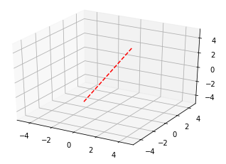
Draw a line between two points
This show how to draw a single line from (-1,-2,-3) to (1,2,3)
|
Filename : Line3D.py |
|
import pandas as pd import numpy as np import matplotlib.pyplot as plt import mpl_toolkits.mplot3d.axes3d as axes3d
fig = plt.figure()
ax = fig.add_subplot(1,1,1, projection='3d')
ax.plot([-1,1],[-2,2],[-3,3],'r--')
ax.set_xlim3d(-5, 5) ax.set_ylim3d(-5, 5) ax.set_zlim3d(-5, 5)
plt.show()
|
| Result : |
|
|
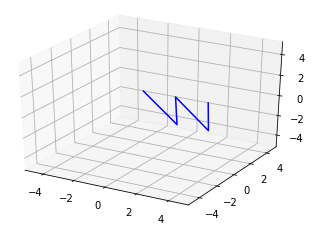
Drawing lines connecting multiple points
This show how to draw the line traces connecting multiple points
|
Filename : Line3D.py |
|
import pandas as pd import numpy as np import matplotlib.pyplot as plt import mpl_toolkits.mplot3d.axes3d as axes3d
fig = plt.figure()
ax = fig.add_subplot(1,1,1, projection='3d')
xList = [0,1,2,3,4] yList = [-1,1,-1,1,-1] zList = [2,-2,2,-2,2]
ax.plot(xList, yList, zList,'b')
ax.set_xlim3d(-5, 5) ax.set_ylim3d(-5, 5) ax.set_zlim3d(-5, 5)
plt.show()
|
| Result : |
|
|
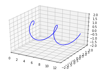
This show how to draw 3d Parameteric Plot
|
Filename : Line3D.py |
|
import pandas as pd import numpy as np import matplotlib.pyplot as plt import mpl_toolkits.mplot3d.axes3d as axes3d
fig = plt.figure()
ax = fig.add_subplot(1,1,1, projection='3d')
t = np.linspace(0, 4 * np.pi, 100) x = t y = np.cos(t) z = np.sin(t)
ax.plot(x, y, z,'b')
ax.set_xlim3d(0, t.max()) ax.set_ylim3d(-2, 2) ax.set_zlim3d(-2, 2)
plt.show()
|
| Result : |
|
|
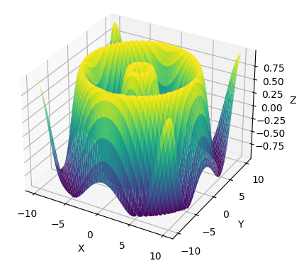
This show how to draw 3d Parameteric Plot
|
Filename : plot3d_surce_01.py |
|
import numpy as np import matplotlib.pyplot as plt
# generate some sample data X, Y = np.meshgrid(np.linspace(-10, 10, 100), np.linspace(-10, 10, 100)) Z = np.sin(np.sqrt(X**2 + Y**2))
# create the plot fig = plt.figure() ax = fig.add_subplot(111, projection='3d') ax.plot_surface(X, Y, Z, cmap='viridis')
# add labels and show the plot ax.set_xlabel('X') ax.set_ylabel('Y') ax.set_zlabel('Z') plt.show()
|
| Result : |
|
|
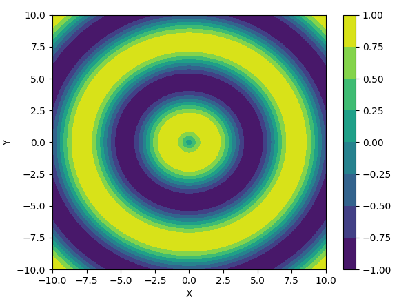
This show how to draw 3d Contour Plot
|
Filename : plot3d_contour_01.py |
|
import numpy as np import matplotlib.pyplot as plt
# generate some sample data X, Y = np.meshgrid(np.linspace(-10, 10, 100), np.linspace(-10, 10, 100)) Z = np.sin(np.sqrt(X**2 + Y**2))
# create the plot fig, ax = plt.subplots()
# plot filled contours c = ax.contourf(X, Y, Z)
# add colorbar and labels cb = fig.colorbar(c) ax.set_xlabel('X') ax.set_ylabel('Y')
plt.show()
|
| Result : |
|
|
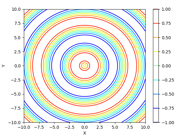
This show how to remove the surface color. Use contour() function instead of contourf().
|
Filename : plot3d_contour_01.py |
|
import numpy as np import matplotlib.pyplot as plt
# generate some sample data X, Y = np.meshgrid(np.linspace(-10, 10, 100), np.linspace(-10, 10, 100)) Z = np.sin(np.sqrt(X**2 + Y**2))
# create the plot fig, ax = plt.subplots()
# plot contours with single color or grayscale colormap plt.contour(X, Y, Z, cmap='jet') plt.colorbar()
# add labels ax.set_xlabel('X') ax.set_ylabel('Y')
plt.show() |
| Result : |
|
|
|
Filename : plot3d_contour_01.py |
|
import numpy as np import matplotlib.pyplot as plt
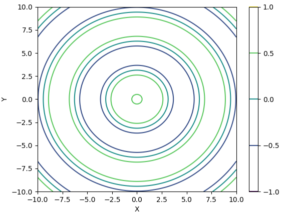
# generate some sample data X, Y = np.meshgrid(np.linspace(-10, 10, 100), np.linspace(-10, 10, 100)) Z = np.sin(np.sqrt(X**2 + Y**2))
# create the plot fig, ax = plt.subplots()
# plot contours with single color or grayscale colormap levels = [-1.0, -0.5, 0, 0.5, 1.0] plt.contour(X, Y, Z, levels=levels) plt.colorbar()
# add labels ax.set_xlabel('X') ax.set_ylabel('Y')
plt.show() |
| Result : |
|
|
|
Filename : plot3d_contour_01.py |
|
import numpy as np import matplotlib.pyplot as plt
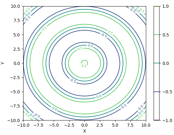
# generate some sample data X, Y = np.meshgrid(np.linspace(-10, 10, 100), np.linspace(-10, 10, 100)) Z = np.sin(np.sqrt(X**2 + Y**2))
# create the plot fig, ax = plt.subplots()
# plot contours with single color or grayscale colormap levels = [-1.0, -0.5, 0, 0.5, 1.0] contours = plt.contour(X, Y, Z, levels=levels) plt.clabel(contours, inline=True, fontsize=8, fmt='%1.1f') plt.colorbar()
# add labels ax.set_xlabel('X') ax.set_ylabel('Y')
plt.show() |
| Result : |
|
|
This show how to format tick mark,tick label,axis label
|
Filename : Line3D.py |
|
import pandas as pd import numpy as np import matplotlib.pyplot as plt import mpl_toolkits.mplot3d.axes3d as axes3d
fig = plt.figure()
ax = fig.add_subplot(1,1,1, projection='3d')
t = np.linspace(0, 4 * np.pi, 100) x = t y = np.cos(t) z = np.sin(t)
ax.plot(x, y, z,'b')
ax.set_xlim3d(0, t.max()) ax.set_ylim3d(-2, 2) ax.set_zlim3d(-2, 2)
ax.set_xlabel('x', fontsize=15, rotation=0) ax.set_ylabel('y', fontsize=15, rotation=0) ax.set_zlabel('z', fontsize=15, rotation=90)
ax.xaxis.set_ticks([0,np.pi,2*np.pi,3*np.pi,4*np.pi]) ax.set_xticklabels([0,'$\pi$','2$\pi$','3$\pi$','4$\pi$'])
ax.yaxis.set_ticks([-2,-1,0,1,2]) ax.zaxis.set_ticks([-2,-1,0,1,2])
plt.show()
|
| Result : |
|
|

Turn Off Axis, Axis Labels, Grid
|
Filename : Line3D.py |
|
import pandas as pd import numpy as np import matplotlib.pyplot as plt import mpl_toolkits.mplot3d.axes3d as axes3d
fig = plt.figure()
ax = fig.add_subplot(1,1,1, projection='3d')
t = np.linspace(0, 4 * np.pi, 100) x = t y = np.cos(t) z = np.sin(t)
ax.plot(x, y, z,'b')
ax.set_xlim3d(0, t.max()) ax.set_ylim3d(-2, 2) ax.set_zlim3d(-2, 2)
ax.set_xlabel('x', fontsize=15, rotation=0) ax.set_ylabel('y', fontsize=15, rotation=0) ax.set_zlabel('z', fontsize=15, rotation=90)
ax.xaxis.set_ticks([0,np.pi,2*np.pi,3*np.pi,4*np.pi]) ax.set_xticklabels([0,'$\pi$','2$\pi$','3$\pi$','4$\pi$'])
ax.yaxis.set_ticks([-2,-1,0,1,2]) ax.zaxis.set_ticks([-2,-1,0,1,2]) ax.grid(False) ax.axis('off') ax.set_xticks([]) ax.set_yticks([]) ax.set_zticks([])
plt.show()
|
| Result : |
|
|

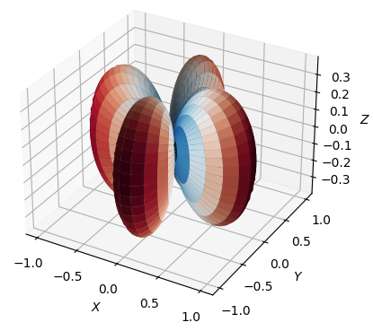
For most of 3D surface plot, you may not need to worry much about the colormap because the default color map would be good enough unless you have any specific preferance of your own. However for the 3D surface plot in spherical coordinate you may want to apply different colormap. In default colormap in 3d surface plot, the surface color changes as the value in Z axis varies, but in spherical plot it would be more meaning to change color of the surface as the value in Radial axis varies. This is an example of showing the color variation along with radial axis (not along with Z axis).
|
Filename : plot3d_spherical_color_01.py |
|
import numpy as np import matplotlib.pyplot as plt import matplotlib.cm as cm from mpl_toolkits.mplot3d import Axes3D
# Generate spherical coordinates phi = np.linspace(0, np.pi, 100) theta = np.linspace(0, 2 * np.pi, 100) PHI, THETA = np.meshgrid(phi, theta) R = (np.sin(PHI) ** 2) * np.cos(2 * THETA)
# Convert spherical coordinates to cartesian coordinates X = R * np.sin(PHI) * np.cos(THETA) Y = R * np.sin(PHI) * np.sin(THETA) Z = R * np.cos(PHI)
# Normalize r for color encoding normalized_r = np.abs(R) normalized_r = (normalized_r - normalized_r.min()) / (normalized_r.max() - normalized_r.min())
# Define a colormap that maps normalized r to red or blue cmap = cm.get_cmap('RdBu_r') colors = cmap(normalized_r)
# Plot the surface fig = plt.figure() ax = fig.add_subplot(111, projection='3d') ax.plot_surface(X, Y, Z, facecolors=colors, linewidth=0) ax.set_xlabel(r'$X$') ax.set_ylabel(r'$Y$') ax.set_zlabel(r'$Z$') plt.show()
|
| Result : |
|
|
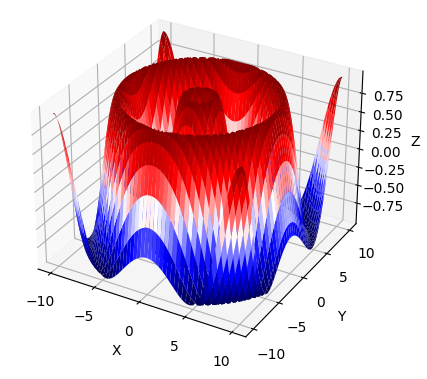
If you apply the color map to cartesian surface plot, it become a little bit simple as below.
|
Filename : plot3d_surce_01_cmap.py |
|
import numpy as np import matplotlib.pyplot as plt
# generate some sample data X, Y = np.meshgrid(np.linspace(-10, 10, 100), np.linspace(-10, 10, 100)) Z = np.sin(np.sqrt(X**2 + Y**2))
# create the plot fig = plt.figure() ax = fig.add_subplot(111, projection='3d')
# create custom colormap cmap = plt.cm.get_cmap('seismic')
# plot surface using custom colormap ax.plot_surface(X, Y, Z, cmap=cmap)
# add labels and show the plot ax.set_xlabel('X') ax.set_ylabel('Y') ax.set_zlabel('Z') plt.show()
|
| Result : |
|
|
If you can change transparency of the surface color as shown below.
|
Filename : plot3d_surce_01_cmap.py |
|
import numpy as np import matplotlib.pyplot as plt
# generate some sample data X, Y = np.meshgrid(np.linspace(-10, 10, 100), np.linspace(-10, 10, 100)) Z = np.sin(np.sqrt(X**2 + Y**2))
# create the plot fig = plt.figure() ax = fig.add_subplot(111, projection='3d')
# plot surface with transparency ax.plot_surface(X, Y, Z, cmap='viridis', alpha=0.5)
# add labels and show the plot ax.set_xlabel('X') ax.set_ylabel('Y') ax.set_zlabel('Z') plt.show()
|
| Result : |
|
|
Reference :
[1] Matplotlib tutorial (Nicolas P. Rougier)