This interactive tutorial visualizes Multi-Head Attention, the extension of single-head attention that allows Transformers to capture different types of relationships simultaneously. In Module 2, we built a single "Filing System" (One Attention Head) that performs Scaled Dot-Product Attention: Q, K, V transformation → Dot Products → Softmax → Weighted Sum. In this module, we show that the Transformer actually runs multiple copies of that exact same Module 2 process in parallel, each with its own learned weight matrices (W_Q,i, W_K,i, W_V,i). Inside every one of these colored lanes, the entire "Filing System" process from Module 2 is happening independently.

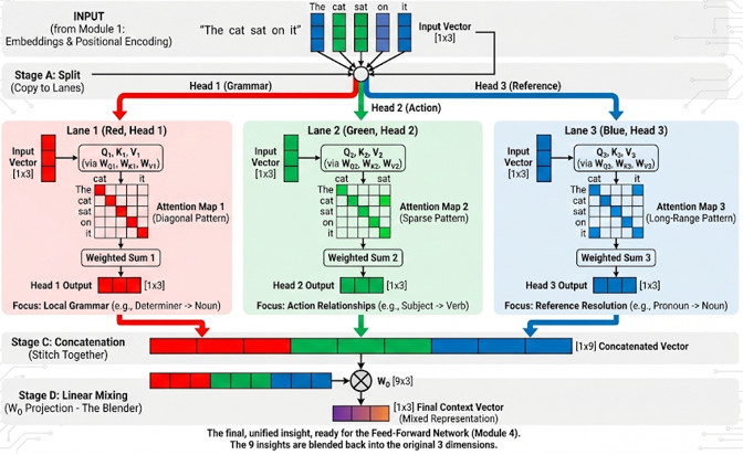
The tutorial demonstrates the complete Multi-Head Attention pipeline: Stage A: Input Embeddings - Output from Module 1 (Embeddings) for the sentence "The cat sat on it", Stage B: Split/Projection - The input is "copied" into multiple lanes (one per head), each with different learned projections (W_Q,i, W_K,i, W_V,i), Stage C: Parallel Attention Maps - Each head performs the exact same Module 2 process (Q, K, V → Dot Products → Softmax → Weighted Sum) independently, but because each head has different learned weights, they learn different relationships (Head 1: Grammar patterns, Head 2: Context/Action relationships, Head 3: Reference/Pronoun resolution), Stage D: Concatenation - Outputs from all heads are stitched together into one long vector, and Stage E: Linear Mixing - Final linear layer (W_O) mixes the concatenated head outputs back to original dimension, producing a rich representation that combines insights from all heads.

The tutorial visualizes 3 Parallel Heads (instead of the standard 8) for screen readability. Each head has distinct attention patterns: Head 1 (Grammar) focuses on immediate neighbors (local grammar patterns like "The" → "cat"), Head 2 (Context/Action) focuses on Subject-Verb relationships (e.g., "cat" → "sat"), and Head 3 (Reference) focuses on Pronoun resolution and long-range dependencies (e.g., "it" → "cat"). The key insight is that different heads learn to focus on different aspects of the input, and their outputs are combined to create a richer representation than any single head could produce alone.

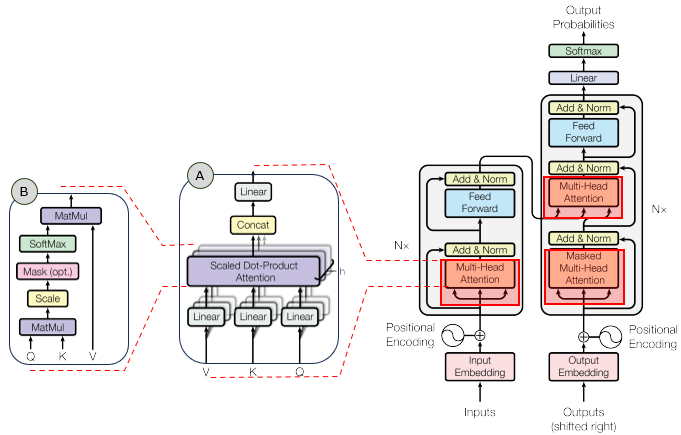
In the overall transformer architecture, this tutorial will cover the blocks highligned in the red box as shown below.

The detailed infographics of this tutorial is as follows.

NOTE : This tutorial uses 3D vectors for visualization clarity. Real Transformers use much higher dimensions (typically d_model = 512 or 768) and 8 or more heads. The tutorial demonstrates Multi-Head Attention where the same input is processed by multiple parallel attention heads, each learning different relationships. The formula for Multi-Head Attention is: MultiHead(Q, K, V) = Concat(head₁, ..., head_h)W_O, where head_i = Attention(QW_Q,i, KW_K,i, VW_V,i). Each head has its own learned weight matrices (W_Q,i, W_K,i, W_V,i), allowing it to learn different types of relationships. The outputs are concatenated and then projected through W_O to produce the final output.

 

Usage Example

Follow these steps to explore how Multi-Head Attention works:

1. Initial State: When you first load the simulation, you'll see the sentence "The cat sat on it" with all 5 tokens processed. The visualization shows five main stages: (A) Input Embeddings (Output from Module 1), (B) Split/Projection (Input → 3 Parallel Heads), (C) Parallel Attention Maps (3 Heads Processing), (D) Concatenation (Stitch Head Outputs Together), and (E) Linear Mixing (W_O Projection). Notice how the same input embeddings are processed by 3 different heads in parallel, each learning different relationships. This demonstrates Multi-Head Attention: multiple "filing systems" working simultaneously to capture different aspects of the input.
2. Stage A: Input Embeddings: The first visualization shows the input embeddings for all 5 tokens in the sentence "The cat sat on it":
   • Each token has an embedding vector (white bars) - these are the output from Module 1 (Embeddings)
   • Shape: [5, d_model] = [5, 3] in this tutorial
   • In real Transformers, these embeddings include word embeddings + positional encodings
   • All 5 tokens are shown side by side to represent the full input sequence
   This demonstrates the starting point: the input embeddings that will be processed by multiple attention heads in parallel.
3. Stage B: Split/Projection: The second visualization shows how the input is "copied" into 3 parallel lanes:
   • The input embeddings are shown at the top (white)
   • Three lanes below represent the 3 heads: Head 1 (Grammar, red), Head 2 (Context, green), Head 3 (Reference, blue)
   • Critical Understanding: Each lane will perform the exact same Module 2 process (Scaled Dot-Product Attention: Q, K, V transformation → Dot Products → Softmax → Weighted Sum)
   • Each head receives the same input but processes it with different learned projections (W_Q,i, W_K,i, W_V,i)
   • In real Transformers, each head has its own W_Q, W_K, W_V matrices (learned during training)
   • Think of it as hiring 3 workers to sit side-by-side, each doing the same job (Module 2) but with different tools (different weight matrices)
   This demonstrates how Multi-Head Attention splits the input into parallel processing lanes, one per head. Each lane is a complete "mini-Module 2" that will run independently.
4. Stage C: Parallel Attention Maps (Each Head = Mini Module 2): The third visualization shows 3 attention heatmaps side by side. Inside each colored lane, the entire Module 2 "Filing System" process is happening:
   • Step 1: Transform to Q, K, V via W_Q,i, W_K,i, W_V,i (each head has different weights)
   • Step 2: Compute Dot Products (Q · K) - measuring similarity
   • Step 3: Apply Softmax - converting scores to attention weights
   • Step 4: Weighted Sum of Values - producing the head output
   • The heatmaps show the final attention weights from this process
   • Head 1 (Grammar, red): Shows diagonal pattern - Head 1's Query asks "Find words that agree with verb tense" (e.g., "The" → "cat", "cat" → "sat")
   • Head 2 (Context/Action, green): Shows sparse pattern - Head 2's Query asks "Find the noun I'm referring to" (e.g., "cat" → "sat")
   • Head 3 (Reference, blue): Shows long-range pattern - Head 3's Query asks "Find the pronoun antecedent" (e.g., "it" → "cat")
   • Each heatmap cell shows attention weight from token i (row) to token j (column)
   • Brighter colors indicate higher attention weights
   • The patterns are different because each head's learned weights (W_Q,i, W_K,i, W_V,i) produce different Queries, which ask different "questions"
   This demonstrates that each head performs the exact same Module 2 process, but with different learned weights, resulting in different attention patterns. The distinct patterns prove that different weights lead to different "questions" being asked.
5. Use Focus Head Buttons: Click the "Focus Head" buttons to isolate specific heads:
   • Show All: Displays all 3 heads simultaneously (default)
   • Focus Head 1: Dims other heads and highlights Head 1 (Grammar) - shows local grammar patterns
   • Focus Head 2: Dims other heads and highlights Head 2 (Context) - shows Subject-Verb relationships
   • Focus Head 3: Dims other heads and highlights Head 3 (Reference) - shows Pronoun resolution
   This allows you to examine each head's behavior in isolation and understand what each head is "looking at".
6. Stage D: Concatenation: The fourth visualization shows how head outputs are stitched together:
   • For each token, the outputs from all 3 heads are concatenated into one long vector
   • Shape: [5, numHeads * d_k] = [5, 9] in this tutorial (3 heads × 3 dimensions each)
   • The concatenated vector is color-coded: red (Head 1), green (Head 2), blue (Head 3)
   • This combines the insights from all heads into a single representation
   This demonstrates the concatenation step: outputs from all heads are combined into one long vector per token.
7. Stage E: Linear Mixing (W_O Projection): The fifth visualization shows the final output after W_O projection:
   • The concatenated vectors are projected through W_O (learned output matrix)
   • Shape: [5, numHeads * d_k] × [numHeads * d_k, d_model] → [5, d_model]
   • This mixes the concatenated head outputs back to the original embedding dimension
   • The final output (purple) is a rich representation that combines insights from all heads
   • This is what gets passed to the next layer of the Transformer
   This demonstrates the final step: the concatenated head outputs are mixed through W_O to produce the final Multi-Head Attention output.
8. Understand the Key Insight: Multi-Head Attention allows the model to capture different types of relationships simultaneously:
   • Single Head: Can only focus on one type of relationship at a time
   • Multiple Heads: Can capture Grammar, Context, Reference, and other relationships in parallel
   • Combination: The final output combines insights from all heads, creating a richer representation
   • This is why Multi-Head Attention is more powerful than single-head attention
   The key insight is that different heads learn to focus on different aspects, and their combination creates a more comprehensive understanding of the input.
9. Observe the Attention Patterns: Look at the attention heatmaps to understand what each head learns:
   • Head 1 (Grammar): Diagonal pattern shows local focus - "The" attends to "cat", "cat" attends to "sat", etc.
   • Head 2 (Context): Sparse pattern shows specific connections - "cat" strongly attends to "sat" (subject-verb)
   • Head 3 (Reference): Long-range pattern shows pronoun resolution - "it" attends to "cat" (resolving the pronoun)
   • Each pattern is distinct, proving that each head learns different relationships
   This demonstrates how Multi-Head Attention captures multiple types of relationships that a single head could not capture alone.
10. Understand the Math: Multi-Head Attention uses:
    • Per-Head Attention: head_i = Attention(QW_Q,i, KW_K,i, VW_V,i)
    • Concatenation: Concat(head₁, ..., head_h) - stitches head outputs together
    • Output Projection: MultiHead = Concat(head₁, ..., head_h)W_O
    • Each head has its own learned weight matrices, allowing it to learn different relationships
    The full formula is: MultiHead(Q, K, V) = Concat(head₁, ..., head_h)W_O, where each head computes attention independently with its own learned projections.

Tip: The key insight is that Multi-Head Attention allows the Transformer to capture multiple types of relationships simultaneously. Instead of one "filing system" (single head), the model uses multiple parallel "filing systems" (multiple heads), each learning to focus on different aspects. Head 1 might learn grammar patterns (local neighbors), Head 2 might learn semantic relationships (subject-verb), and Head 3 might learn long-range dependencies (pronoun resolution). The outputs from all heads are concatenated and then mixed through W_O to produce a rich final representation. Use the "Focus Head" buttons to examine each head's behavior in isolation - notice how each head's attention pattern is distinct, proving that each head learns different relationships. This is why Multi-Head Attention is more powerful than single-head attention: it can capture multiple types of relationships in parallel, creating a more comprehensive understanding of the input.

Description on Stages

This section provides detailed descriptions of each stage in the Multi-Head Attention pipeline:

• Stage A: Input Embeddings (Output from Module 1): The starting point of Multi-Head Attention. This stage displays the input embeddings for all 5 tokens in the sentence "The cat sat on it". Each token has an embedding vector with shape [d_model] = [3] in this tutorial. These embeddings are the output from Module 1 (Embeddings), which combine word embeddings with positional encodings. The embeddings are displayed as white vertical bar charts, with each bar representing one dimension. All tokens are shown side by side to represent the full input sequence. Shape: [numTokens, d_model] = [5, 3]. This stage explicitly labels the input as "Output from Module 1" to reinforce the pipeline mental model, showing how Multi-Head Attention fits into the larger Transformer architecture.
• Stage B: Split/Projection (Input → 3 Parallel Heads): This stage shows how the input embeddings are "copied" into 3 parallel lanes, one for each attention head. The input embeddings are shown at the top (white), and three lanes below represent the 3 heads, each color-coded: Head 1 (Grammar, red), Head 2 (Context/Action, green), Head 3 (Reference, blue). Key Insight: Each lane will perform the exact same Module 2 process (Scaled Dot-Product Attention: Q, K, V transformation → Dot Products → Softmax → Weighted Sum), but with different learned weight matrices (W_Q,i, W_K,i, W_V,i). Think of it as hiring 3 workers to sit side-by-side, each doing the same job (Module 2) but with different tools (different weight matrices). Each head receives the same input but processes it with different learned projections. In real Transformers, each head has its own W_Q, W_K, W_V matrices that are learned during training. The visualization includes a label "← Mini Module 2 (Same Process)" under each head lane to emphasize this connection.
• Stage C: Parallel Attention Maps (Each Head = Mini Module 2): This stage displays 3 attention heatmaps side by side, one for each head. Important Clarification: These heatmaps visualize the output of Step 4 (Softmax / Attention Weights), not the final output of Step 6. The matrix represents the "map of attention" (the recipe for how to mix), not the final cooked result.
  • Data Shape: [numTokens, numTokens] = [5, 5] - a square grid where each cell represents a relationship between two words
  • What it holds: Probabilities (0.0 to 1.0) - attention weights after Softmax normalization
  • Purpose: It tells you how much to mix. It is the "recipe" for combining Values in Step 6
  How to Calculate This Matrix (The Module 2 Process): Inside each colored lane, the entire Module 2 "Filing System" process is happening independently:
  1. Create Q and K: The input sentence ("The cat sat on it") is converted into vectors. Each head applies its specific weight matrices (W_Q,i, W_K,i) to create a Query vector and a Key vector for every word. For example, Head 1 applies W_Q,1 and W_K,1 to create Queries and Keys.
  2. The Dot Product (Q · K): The model multiplies every Query (row) against every Key (column). For example, it multiplies the Query vector for "The" against the Key vector for "cat". If they are mathematically similar, the result is a high number (e.g., 5.0). This produces raw similarity scores.
  3. Scaling & Softmax: The raw scores are divided by a scaling factor (√d_k) and passed through a Softmax function. Crucial Math Check: Softmax forces the numbers in each Row to sum up to exactly 1.00 (or 100%). For example, in the first row ("The"), all attention weights must sum to 1.0. The values you see in the heatmap are these final probabilities.
  4. Weighted Sum of Values (Step 6): After obtaining the attention weights (shown in the heatmap), the model uses these weights to compute a weighted sum of Values. This produces the final head output, which has shape [numTokens, d_k] (not shown in the heatmap, but visualized in Stage D as concatenated outputs).
  How to Interpret Each Element (Reading the Grid): Think of this matrix as a map of "Who is looking at whom?"
  • The Rows (Y-Axis) = The Observer (Query): This represents the word currently being processed. "I am the word 'The'..."
  • The Columns (X-Axis) = The Target (Key): This represents the context being looked at. "...and I am looking at 'cat'."
  • The Cell Value = The Attention Intensity: This number tells you how much "focus" the Observer is placing on the Target. It ranges from 0.0 (no attention) to 1.0 (100% attention).
  Concrete Examples from Head 1 (Grammar Pattern):
  • Case A: Cell (Row: "The", Col: "cat") = 0.80 - Interpretation: When the model tries to understand the word "The", it spends 80% of its mental energy looking at the word "cat". Why? In English grammar, a determiner ("The") is meaningless without the noun it points to ("cat"). This Head has learned that "The" should always look at the next word.
  • Case B: Cell (Row: "cat", Col: "sat") = 0.50 - Interpretation: When processing the word "cat", the model pays 50% attention to "sat". Why? To understand the subject ("cat"), it helps to know the verb ("sat")—"Who is the cat? The one that sat."
  • Case C: The Zeros (0.00) - Interpretation: "The" pays 0.00 attention to "sat". Why? The word "sat" is too far away or grammatically irrelevant to the word "The" at this specific moment.
  The "Pattern" of Each Head: If you examine the heatmaps, you'll see distinct visual patterns that prove each head learns different relationships:
  • Head 1 (Grammar, red): The bright red blocks form a pattern that is mostly one step to the right of the diagonal. Diagonal: (The, The), (cat, cat), (sat, sat)... Head 1's Focus: (The, cat), (cat, sat), (sat, on)... This visual pattern proves that Head 1 acts like a "Next Word Detector," focusing on immediate neighbors (local grammar patterns).
  • Head 2 (Context/Action, green): Shows a sparse pattern - focuses on Subject-Verb relationships (e.g., "cat" → "sat"). The pattern is less uniform, indicating selective attention to specific grammatical relationships.
  • Head 3 (Reference, blue): Shows a long-range pattern - focuses on Pronoun resolution (e.g., "it" → "cat"). The pattern shows connections that span across the sentence, indicating long-range dependency resolution.
  Why Different Patterns? The patterns are different because each head's learned weights (W_Q,i, W_K,i, W_V,i) produce different Queries, which ask different "questions". Head 1's Query might mathematically translate to "Find words that agree with verb tense" (Grammar), Head 2's Query might translate to "Find the noun I'm referring to" (Context), and Head 3's Query might translate to "Find the pronoun antecedent" (Reference). Same process, different "questions" being asked. The visualization includes a label "Module 2 Process: Q,K,V → Dot Products → Softmax → Weighted Sum" above each attention map to reinforce this connection.
• Stage D: Concatenation (Stitch Head Outputs Together): This stage shows how the outputs from all 3 heads are concatenated (stitched together) into one long vector for each token. Understanding the Dimensionality: Each head produces a [1×3] vector (3 dimensions) for each token. Here's how that dimensionality is created inside each head:
  • The Source: The Value Weight Matrix (W_V,i): The size of the output vector for a Head is determined entirely by the shape of its Value Weight Matrix (W_V,i). You start with the embedding for a word (e.g., "The"), which is a vector of size [1×3]. Inside Head 1, this input is multiplied by W_V,1. If W_V,1 is a [3×3] matrix, the math is: [1×3] × [3×3] = [1×3]. Result: You get a Value Vector (V) that is size [1×3].
  • The Mixing: Weighted Sum: Next, the Attention Mechanism (the attention matrix from Stage C) calculates the weighted sum: Σ(Attention Weight × Value). The Dimensionality: When you add two vectors of size [1×3], the result is still a vector of size [1×3]. Analogy: If you mix a 3-gallon bucket of red paint with a 3-gallon bucket of white paint, you still have a bucket with 3-gallon capacity. You don't suddenly get a 6-gallon bucket or a 1-gallon bucket. The "shape" of the data container doesn't change during addition. This weighted sum produces the final head output, which is [1×3] for each token.
  The Concatenation Process: For each token (e.g., "The"), here's what happens:
  • Head 1 (Grammar) finishes its math and spits out a Red [1×3] vector
  • Head 2 (Context/Action) finishes its math and spits out a Green [1×3] vector
  • Head 3 (Reference) finishes its math and spits out a Blue [1×3] vector
  The Concatenation: The model takes these three vectors and stitches them together: [1×3] + [1×3] + [1×3] → [1×9]. For the full sequence of 5 tokens, the shape is [numTokens, numHeads × d_k] = [5, 9] in this tutorial (3 heads × 3 dimensions each). The concatenated vector is color-coded: red (Head 1), green (Head 2), blue (Head 3). This visualization shows how insights from all heads are combined into a single representation per token. The concatenation step is crucial because it preserves the information from all heads before the final mixing step. Each token's concatenated vector contains the output from all heads, allowing the model to combine different types of relationships (Grammar, Context, Reference) into one comprehensive representation. Technical Note: In real-world Transformers (like GPT-3), they usually split the dimensions to keep the math smaller. Real World: Input is 512. 8 Heads. Each head projects down to size 64 (d_k = 512/8 = 64). Concatenation is [numTokens, 512]. Your Tutorial: Input is 3. 3 Heads. Each head stays at size 3 (for visibility). Concatenation is [numTokens, 9]. The final linear layer (W_O) will shrink it back to [numTokens, 3] in Stage E.
• Stage E: Linear Mixing (W_O Projection): This stage shows the final output after applying the output projection matrix W_O. This stage is the compression and blending step that transforms the concatenated head outputs back to the original embedding dimension. How is this obtained? (The Math):
  • The Input (from Stage D): Recall the previous step (Concatenation). For each word (e.g., "The"), you had a long vector made of 3 parts stitched together: [Head 1 Output] + [Head 2 Output] + [Head 3 Output]. Size: 3 dims + 3 dims + 3 dims = 9 dimensions. For the full sequence of 5 tokens, the shape is [5, 9].
  • The Mechanism (W_O): The model has a final learned matrix called W_O (Output Weights). Matrix Shape: [9 × 3] (It maps 9 inputs to 3 outputs). This matrix is learned during training and determines how to mix insights from different heads.
  • The Calculation: The model performs a matrix multiplication: [numTokens, 9] × [9, 3] = [numTokens, 3]. For example, [5, 9] × [9, 3] = [5, 3]. The math successfully squashes the 9-dimensional combined insights back down to the original 3-dimensional size (d_model = 3).
  • The Result: You see a vector with 3 bars (d0, d1, d2) for each token. Each token's output is displayed as a purple vector with three bars (one per dimension). The purple color distinguishes this final output from the intermediate head outputs.
  How to Interpret It (The Intuition): Think of this vector as a "Context-Aware Smoothie."
  • Stage C (Attention Maps): Was like gathering separate ingredients. Head 1 found the grammar ingredient, Head 2 found the subject ingredient, Head 3 found the reference ingredient.
  • Stage D (Concatenation): Was putting all those ingredients side-by-side in a bowl. You could still see them separately (red, green, blue segments).
  • Stage E (Linear Mixing): Is the blender. The W_O matrix mixes all those separate insights together into one unified representation.
  What do the specific values mean? Look at the result for a word like "cat":
  • Example values: [-0.09, 0.14, -0.27]
  • Meaning: This is no longer just the dictionary definition of "cat." It contains the "Grammar" info (from Head 1) that "cat" is the object of "The". It contains the "Action" info (from Head 2) that "cat" is the thing doing the "sitting." It contains the "Reference" info (from Head 3) that "cat" might be referenced by "it."
  • Each dimension now represents a blended combination of insights from all three heads, not just a single aspect.
  Why do we shrink it back to 3 dimensions? You might ask, "Why not keep all 9 dimensions? Isn't more data better?" We shrink it back to 3 (d_model) for compatibility. The next component in the Transformer (the Feed-Forward Network, Module 4) expects an input of size 3. By projecting it back to the original size, we allow these blocks to be stacked. The output of Block 1 becomes the valid input for Block 2. This enables the Transformer architecture to be modular and composable. Summary: This stage represents the final, unified thought for each word after one round of Multi-Head Attention. It is the packet of data ready to be sent to the next stage. The final output combines insights from all heads into a rich representation that captures multiple types of relationships simultaneously. This is the final Multi-Head Attention output that gets passed to the next layer of the Transformer.

Parameters

Followings are short descriptions on each parameter

• Input Embeddings: The input to Multi-Head Attention is a sequence of embeddings for the sentence "The cat sat on it" (5 tokens). Shape: [5, d_model] = [5, 3] in this tutorial. These embeddings are the output from Module 1 (Embeddings), which include word embeddings + positional encodings. In real Transformers, d_model = 512 or 768. Each token is displayed as a white vector with three bars (one per dimension). The embeddings are processed by all heads in parallel.
• Number of Heads (numHeads): The number of parallel attention heads. This tutorial uses 3 heads (instead of the standard 8) for screen readability. Each head processes the same input independently with different learned weight matrices. Head 1 (Grammar, red) focuses on local grammar patterns, Head 2 (Context/Action, green) focuses on Subject-Verb relationships, Head 3 (Reference, blue) focuses on Pronoun resolution. In real Transformers, typically 8 or 16 heads are used.
• Head Dimension (d_k): The dimension of each head's output. In this tutorial, d_k = d_model = 3 for simplicity. In real Transformers, d_k = d_model / numHeads (e.g., if d_model = 512 and numHeads = 8, then d_k = 64). This ensures that the concatenated head outputs have the same total dimension as the input (numHeads × d_k = d_model).
• Per-Head Weight Matrices (W_Q,i, W_K,i, W_V,i): Each head has its own learned weight matrices. Head i has W_Q,i (Query weights), W_K,i (Key weights), and W_V,i (Value weights). These matrices are learned during training and allow each head to learn different relationships. In this tutorial, the attention patterns are hardcoded to demonstrate distinct behaviors, but in real Transformers, these patterns emerge from learned weights.
• Attention Patterns: Each head has a distinct attention pattern (hardcoded for visualization):
  • Head 1 (Grammar): Diagonal pattern - focuses on immediate neighbors (local grammar)
  • Head 2 (Context/Action): Sparse pattern - focuses on Subject-Verb relationships
  • Head 3 (Reference): Long-range pattern - focuses on Pronoun resolution
  Each pattern is a [numTokens, numTokens] matrix where entry [i, j] is the attention weight from token i to token j. The patterns are normalized so each row sums to 1.0.
• Head Outputs: Each head produces an output for each token by computing a weighted sum of all tokens based on its attention pattern. Shape: [numTokens, d_k] = [5, 3] per head. The output for token i is computed as: output[i] = Σ_j(attention[i, j] × input[j]). This is the result of applying attention within each head.
• Concatenation: The outputs from all heads are concatenated along the feature dimension. Shape: [numTokens, numHeads × d_k] = [5, 9] in this tutorial (3 heads × 3 dimensions). For each token, the outputs from all heads are stitched together into one long vector. This combines insights from all heads into a single representation.
• Output Projection Matrix (W_O): A learned matrix that projects the concatenated head outputs back to the original embedding dimension. Shape: [numHeads × d_k, d_model] = [9, 3] in this tutorial. This matrix mixes the concatenated head outputs to produce the final Multi-Head Attention output. The projection allows the model to learn how to combine insights from different heads.
• Final Output: The result of Multi-Head Attention after W_O projection. Shape: [numTokens, d_model] = [5, 3] in this tutorial. This is a rich representation that combines insights from all heads. Each token's output is a weighted combination of information from all tokens, where the weights come from multiple attention heads that learned different relationships.
• Embedding Dimension (d_model): The dimension of input embeddings and final output (3 in this tutorial for visualization, but 512+ in real Transformers). All input and output vectors have dimension d_model. The head dimension d_k is typically d_model / numHeads to ensure the concatenated outputs have the same total dimension as the input.
• Multi-Head Attention Formula: The full Multi-Head Attention mechanism: MultiHead(Q, K, V) = Concat(head₁, ..., head_h)W_O, where head_i = Attention(QW_Q,i, KW_K,i, VW_V,i). Each head computes scaled dot-product attention independently with its own learned projections, then all head outputs are concatenated and projected through W_O to produce the final output.

Controls and Visualizations

Followings are short descriptions on each control and visualization

• Focus Head Buttons: Four buttons to control which heads are displayed: [Show All] [Focus Head 1] [Focus Head 2] [Focus Head 3]. "Show All" displays all 3 heads simultaneously (default). When a specific head is focused, the other heads are dimmed (opacity reduced) and the focused head is highlighted. This allows you to examine each head's behavior in isolation and understand what each head is "looking at". The active button is highlighted in green.
• Input Embeddings Canvas: Canvas-based vertical bar charts showing the input embeddings for all 5 tokens in the sentence "The cat sat on it". Each token is displayed as a white vector with three bars (one per dimension). The embeddings are labeled with the actual words ("The", "cat", "sat", "on", "it"). These embeddings are the output from Module 1 (Embeddings) and serve as the input to Multi-Head Attention. Shape: [5, d_model] = [5, 3].
• Split/Projection Visualization: A visual representation showing how the input is "copied" into 3 parallel lanes (one per head). The input embeddings are shown at the top (white). Three lanes below represent the 3 heads, each color-coded: Head 1 (Grammar, red), Head 2 (Context, green), Head 3 (Reference, blue). Each head receives the same input but processes it with different learned projections. When a head is focused, other lanes are dimmed.
• Attention Maps Canvas: Three Canvas-based heatmaps showing the attention patterns for each head. Each heatmap is a [numTokens, numTokens] grid where cell [i, j] shows the attention weight from token i (row) to token j (column). Brighter colors indicate higher attention weights. Head 1 (Grammar, red) shows a diagonal pattern (local focus), Head 2 (Context, green) shows a sparse pattern (Subject-Verb), Head 3 (Reference, blue) shows a long-range pattern (Pronoun resolution). The distinct patterns prove that each head learns different relationships. When a head is focused, other heatmaps are dimmed.
• Concatenation Canvas: Canvas-based horizontal bar charts showing the concatenated head outputs for each token. For each token, the outputs from all 3 heads are stitched together into one long vector. The concatenated vector is color-coded: red (Head 1), green (Head 2), blue (Head 3). Shape: [numTokens, numHeads × d_k] = [5, 9] in this tutorial. This visualization shows how insights from all heads are combined into a single representation per token.
• Linear Mixing (W_O) Canvas: Canvas-based vertical bar charts showing the final output after W_O projection. Each token's output is displayed as a purple vector with three bars. This is the result of projecting the concatenated head outputs through W_O back to the original embedding dimension. Shape: [numTokens, d_model] = [5, 3]. This is the final Multi-Head Attention output that gets passed to the next layer of the Transformer. The output combines insights from all heads into a rich representation.

Key Concepts and Implementation

This tutorial demonstrates how Multi-Head Attention works, which extends single-head attention to capture multiple types of relationships simultaneously. Here are the key concepts:

• Why Multi-Head Attention is Needed: Single-head attention can only focus on one type of relationship at a time. Multi-Head Attention allows the model to capture multiple types of relationships simultaneously (Grammar, Context, Reference, etc.) by running multiple attention heads in parallel. Each head learns to focus on different aspects of the input, and their outputs are combined to create a richer representation than any single head could produce alone. This is why Multi-Head Attention is more powerful than single-head attention.
• Multi-Head Attention Architecture: Multi-Head Attention consists of:
  • Input Embeddings: The input sequence (e.g., "The cat sat on it") - Shape: [numTokens, d_model]
  • Multiple Parallel Heads: Each head processes the same input independently, performing the exact same Module 2 process (Scaled Dot-Product Attention) but with different learned weight matrices
  • Per-Head Attention: Each head computes scaled dot-product attention: head_i = Attention(QW_Q,i, KW_K,i, VW_V,i). This is the same formula from Module 2, just with head-specific weights. Inside each head: (1) Transform to Q, K, V via W_Q,i, W_K,i, W_V,i, (2) Compute Dot Products (Q · K), (3) Apply Softmax, (4) Weighted Sum of Values
  • Why Different Results?: Because each head has different learned weights (W_Q,i, W_K,i, W_V,i), they produce different Queries. Head 1's Query might mathematically translate to "Find words that agree with verb tense" (Grammar), Head 2's Query might translate to "Find the noun I'm referring to" (Context), Head 3's Query might translate to "Find the pronoun antecedent" (Reference). Same process, different "questions" being asked.
  • Concatenation: Head outputs are concatenated: Concat(head₁, ..., head_h)
  • Output Projection: Concatenated outputs are projected through W_O: MultiHead = Concat(head₁, ..., head_h)W_O
  Each head performs the exact same mathematical process from Module 2, but with different learned weight matrices, allowing it to learn different relationships. The outputs are combined to create a comprehensive representation.
• Multi-Head Attention Formula: The full Multi-Head Attention mechanism:
  • Per-Head Attention: head_i = Attention(QW_Q,i, KW_K,i, VW_V,i)
  • Concatenation: Concat(head₁, ..., head_h) - stitches head outputs together
  • Output Projection: MultiHead = Concat(head₁, ..., head_h)W_O
  Full formula: MultiHead(Q, K, V) = Concat(head₁, ..., head_h)W_O where each head computes scaled dot-product attention independently with its own learned projections.
• Why Multiple Heads Learn Different Relationships: Each head performs the exact same Module 2 process (Scaled Dot-Product Attention), but each head has its own learned weight matrices (W_Q,i, W_K,i, W_V,i), which are learned during training via backpropagation. Because the weights are different, each head produces different Queries. Head 1's Query (computed via W_Q,1) might mathematically translate to "Find words that agree with verb tense" (Grammar), Head 2's Query (computed via W_Q,2) might translate to "Find the noun I'm referring to" (Context), Head 3's Query (computed via W_Q,3) might translate to "Find the pronoun antecedent" (Reference). Same process, different "questions" being asked. Different initializations and training dynamics cause different heads to specialize in different types of relationships. The distinct attention patterns in this tutorial demonstrate this specialization.
• Head Dimension (d_k): In real Transformers, d_k = d_model / numHeads to ensure the concatenated head outputs have the same total dimension as the input. For example, if d_model = 512 and numHeads = 8, then d_k = 64. This ensures that numHeads × d_k = d_model, so the concatenated outputs have shape [numTokens, d_model], matching the input dimension. In this tutorial, d_k = d_model = 3 for simplicity.
• Concatenation and Output Projection: After all heads compute attention independently, their outputs are concatenated along the feature dimension. This creates a long vector per token that combines insights from all heads. The concatenated outputs are then projected through W_O (learned output matrix) back to the original embedding dimension. This projection allows the model to learn how to mix insights from different heads to produce the final output.
• Visual Connection to Module 1: The input embeddings are explicitly labeled as "Output from Module 1 (Embeddings)" to reinforce the pipeline mental model. This shows how Multi-Head Attention fits into the larger Transformer architecture: Embeddings → Multi-Head Attention → Feed-Forward → ... The tutorial demonstrates how embeddings are processed by multiple attention heads in parallel.
• Why 3 Heads Instead of 8: Real Transformers typically use 8 or 16 heads, but this tutorial uses 3 heads for screen readability. With 8 heads, the visualizations become too small to see clearly. The 3 heads (Grammar, Context, Reference) are sufficient to demonstrate the key concept: different heads learn different relationships, and their outputs are combined to create a richer representation.
• What to Look For: When exploring the tutorial, observe: (1) How each head's attention pattern is distinct (diagonal vs. sparse vs. long-range), (2) How the attention heatmaps show different relationships (Grammar, Context, Reference), (3) How head outputs are concatenated into one long vector per token, (4) How the concatenated outputs are projected through W_O to produce the final output, (5) How the final output combines insights from all heads, (6) How focusing on a specific head dims others and highlights that head's behavior. This demonstrates how Multi-Head Attention captures multiple types of relationships simultaneously, creating a more comprehensive understanding of the input than single-head attention.