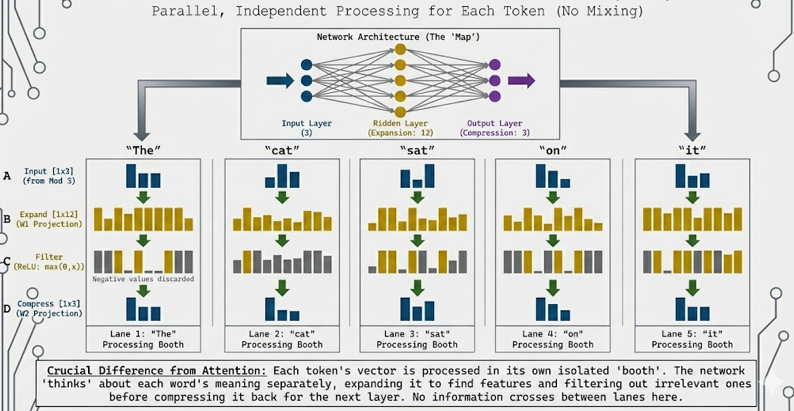
This interactive tutorial visualizes the Feed-Forward Network (FFN), a crucial component of Transformers that processes each token independently. Conceptual Contrast: While Module 3 (Multi-Head Attention) was about "mixing" information between words ("The" talked to "cat"), Module 4 (FFN) is about processing each word individually. Each token goes into its own "isolation booth" - no talking allowed between tokens. This is the key difference: Attention mixes information across the sequence, while FFN processes each position independently.

The tutorial demonstrates the complete FFN pipeline: Stage 0: Network Architecture - A classic "stick and ball" neural network diagram showing the structure (3 input nodes → 12 hidden nodes → 3 output nodes) with connections, Stage A: Input - Context vectors from Module 3 (Multi-Head Attention output) for the sentence "The cat sat on it", Stage B: Expansion - Linear projection that expands each token's representation from d_model = 3 to d_ff = 12 (4× expansion), Stage C: Filter (ReLU Activation) - Non-linear activation that "filters" the expanded representation by zeroing out negative values (discarding irrelevant concepts), and Stage D: Compression - Linear projection that compresses the filtered representation back from d_ff = 12 to d_model = 3. The FFN applies the same transformation to every token, but processes them in parallel isolation.

The tutorial visualizes the Expand → Filter → Compress mechanism. The expansion (3 → 12) creates a richer representation space where the model can learn complex features. The ReLU filter acts as a decision mechanism, keeping only positive (relevant) features and discarding negative (irrelevant) ones. The compression (12 → 3) projects back to the original dimension, maintaining compatibility with the next layer. This process happens independently for each token - "The" is processed in its own lane, "cat" in another, etc., with no information crossing between them.

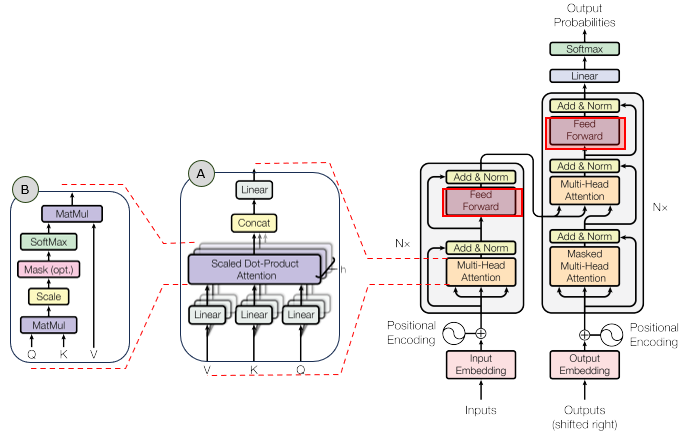
In the overall transformer architecture, this tutorial will cover the blocks highligned in the red box as shown below.

The detailed infographics of this tutorial is as follows.

NOTE : This tutorial uses 3D vectors for visualization clarity. Real Transformers use much higher dimensions (typically d_model = 512 or 768, d_ff = 2048 or 3072, giving a 4× expansion). The tutorial demonstrates the Feed-Forward Network where each token is processed independently through two linear transformations with a ReLU activation in between. The formula is: FFN(x) = max(0, xW₁ + b₁)W₂ + b₂, where W₁ is [d_model, d_ff] (expansion), W₂ is [d_ff, d_model] (compression), and max(0, ·) is the ReLU activation. The key insight is that FFN processes each position independently (unlike Attention which mixes across positions), allowing the model to learn position-specific transformations while maintaining the same architecture for all positions.

 

Usage Example

Follow these steps to explore how the Feed-Forward Network works:

1. Initial State: When you first load the simulation, you'll see the "Show All" view displaying all 5 tokens ("The", "cat", "sat", "on", "it") being processed in parallel lanes. Each token is processed independently in its own "isolation booth" - no information crosses between tokens. When you select a specific token, the visualization shows five main stages: (0) Network Architecture (the structural diagram), (A) Input (Output from Module 3), (B) Expansion (3 → 12 dimensions), (C) Filter (ReLU activation), and (D) Compression (12 → 3 dimensions). Notice how each token goes through the same transformation independently.
2. Stage 0: Network Architecture (The 'Map' of the FFN): When you select a specific token, the visualization begins with a classic "stick and ball" neural network diagram that shows the structure of the FFN:
   • Input Layer: 3 cyan nodes representing the input dimensions (d_model = 3)
   • Hidden Layer: 12 yellow nodes representing the expanded dimensions (d_ff = 12, 4× expansion)
   • Output Layer: 3 purple nodes representing the compressed output dimensions (d_model = 3)
   • Connections: Semi-transparent white lines showing all connections between layers (fully connected network)
   • This diagram provides a visual "map" of the network structure before showing the data flow
   • The diagram is centered and clearly shows the narrow → wide → narrow (bottleneck) architecture
   This demonstrates the structural architecture of the FFN, making the expansion and compression visually clear before the data transformation stages.
3. Stage A: Input (Output from Module 3): The input to the FFN is the context vectors from Module 3 (Multi-Head Attention output):
   • Each token has a context vector (cyan bars) - these are the output from Module 3
   • Shape: [1, d_model] = [1, 3] per token, [5, 3] for all tokens
   • These vectors contain information that was mixed from other tokens via Attention
   • Now, each token will be processed independently - no more mixing
   This demonstrates the starting point: context vectors that will be processed individually by the FFN.
4. Stage B: Expansion (Linear Projection 1): The first linear transformation expands each token's representation:
   • Input: [1, 3] → Output: [1, 12] (4× expansion)
   • Operation: xW₁ + b₁, where W₁ is [3, 12]
   • Visual: 3 cyan bars expand to 12 yellow bars
   • The expansion creates a richer representation space where the model can learn complex features
   • This happens independently for each token - "The" expands in its own lane, "cat" in another, etc.
   This demonstrates the expansion step: each token's representation grows from 3 to 12 dimensions, creating more space for feature learning.
5. Stage C: Filter (ReLU Activation): The non-linear activation function "filters" the expanded representation:
   • Operation: ReLU(x) = max(0, x) - any negative value becomes 0
   • Visual: Yellow bars with negative values turn grey (flattened to 0)
   • Positive bars stay bright yellow
   • Key Insight: ReLU acts as a "filter" that discards negative/irrelevant concepts
   • This is the decision-making step - the network decides which expanded features to keep and which to kill
   • The non-linearity is crucial - without it, the FFN would just be two linear transformations (which is still linear)
   This demonstrates the filtering step: ReLU zeroes out negative values, keeping only positive (relevant) features. This is what makes the FFN non-linear and allows it to learn complex transformations.
6. Stage D: Compression (Linear Projection 2): The second linear transformation compresses the filtered representation back:
   • Input: [1, 12] → Output: [1, 3] (compression back to original size)
   • Operation: yW₂ + b₂, where W₂ is [12, 3]
   • Visual: 12 yellow/grey bars compress to 3 purple bars
   • Only the active (positive) features from Stage C contribute to the output
   • The compression maintains compatibility with the next layer (d_model = 3)
   This demonstrates the compression step: the filtered representation is projected back to the original dimension, maintaining compatibility while preserving the learned features.
7. Use Token Selector: Click the token buttons to focus on a specific word:
   • Show All: Displays all 5 tokens in parallel lanes (default) - shows that FFN processes all tokens simultaneously but independently
   • "The": Focuses on the first token - shows its individual expansion/filter/compression process
   • "cat": Focuses on the second token - shows how "cat" is processed in isolation
   • "sat", "on", "it": Each token button shows that word's individual processing
   This allows you to examine each token's processing in detail. Notice that each token goes through the same transformation, but with different input values, producing different outputs. This demonstrates the "isolation booth" concept - each token is processed independently.
8. Understand the Key Contrast with Module 3: The fundamental difference between Attention and FFN:
   • Module 3 (Attention): "The" talked to "cat" - information mixed between tokens
   • Module 4 (FFN): "The" goes into its own isolation booth - no talking allowed
   • Attention: Processes relationships between tokens (mixing information)
   • FFN: Processes each token individually (no mixing between tokens)
   • Both are necessary: Attention captures context, FFN processes individual representations
   The key insight is that Attention and FFN serve complementary roles: Attention mixes information across the sequence, while FFN processes each position independently.
9. Observe the Expand → Filter → Compress Pattern: Notice the visual pattern in each token's processing:
   • Expand (3 → 12): Creates more space for learning complex features
   • Filter (ReLU): Discards irrelevant features (negative values become 0)
   • Compress (12 → 3): Projects back to original dimension, keeping only the important features
   • This pattern is identical for every token, but each token produces different results based on its input
   This demonstrates the standard FFN architecture: expansion creates learning space, ReLU filters features, compression maintains compatibility.
10. Understand the Math: The FFN formula is:
    • Step 1 (Expansion): h = xW₁ + b₁ where W₁ is [d_model, d_ff]
    • Step 2 (Filter): a = ReLU(h) = max(0, h)
    • Step 3 (Compression): y = aW₂ + b₂ where W₂ is [d_ff, d_model]
    • Full Formula: FFN(x) = max(0, xW₁ + b₁)W₂ + b₂
    • The ReLU activation is crucial - it makes the transformation non-linear, allowing the model to learn complex patterns
    The full formula shows how expansion, filtering, and compression work together to transform each token's representation independently.

Tip: The key insight is the contrast between Module 3 (Attention) and Module 4 (FFN). Attention mixes information between tokens ("The" talked to "cat"), while FFN processes each token individually ("The" goes into its own isolation booth). The FFN uses an Expand → Filter → Compress pattern: (1) Expand from 3 to 12 dimensions to create learning space, (2) Filter with ReLU to discard irrelevant features (negative values become 0), (3) Compress back to 3 dimensions to maintain compatibility. This process happens independently for each token - no information crosses between tokens. Use the token selector to focus on individual words and see how each token is processed in isolation. Notice that the same transformation is applied to every token, but each produces different results based on its input. This demonstrates that FFN processes positions independently, in contrast to Attention which mixes information across positions.

Description on Stages

This section provides detailed descriptions of each stage in the Feed-Forward Network pipeline:

• Stage 0: Network Architecture (The 'Map' of the FFN): This stage displays a classic "stick and ball" neural network diagram that visualizes the structure of the Feed-Forward Network. The diagram appears at the top when you select a specific token for detailed inspection. Visual Elements:
  • Input Layer: 3 cyan-colored circular nodes stacked vertically, representing the input dimensions (d_model = 3)
  • Hidden Layer: 12 yellow-colored circular nodes stacked vertically, representing the expanded dimensions (d_ff = 12, showing the 4× expansion)
  • Output Layer: 3 purple-colored circular nodes stacked vertically, representing the compressed output dimensions (d_model = 3)
  • Connections: Semi-transparent white lines (rgba(255, 255, 255, 0.1)) connecting every input node to every hidden node, and every hidden node to every output node, showing a fully connected (dense) network structure
  • Layout: The diagram is horizontally centered and clearly shows the narrow → wide → narrow (bottleneck) architecture pattern
  Purpose: This diagram provides a visual "map" of the network structure before showing the data flow. It grounds the abstract "Vector Expansion" concept in the familiar "Neural Network" visual language, making the structural relationship between layers immediately clear. The diagram makes the expansion (3 → 12) and compression (12 → 3) explicitly visible as a shape, helping students understand the architecture before seeing the data transformations.
• Stage A: Input (Output from Module 3): The starting point of the Feed-Forward Network. This stage displays the context vectors for all 5 tokens in the sentence "The cat sat on it". Each token has a context vector with shape [d_model] = [3] in this tutorial. These vectors are the output from Module 3 (Multi-Head Attention), which contain information that was mixed from other tokens via Attention. The vectors are displayed as cyan vertical bar charts, with each bar representing one dimension. The bars are scaled to be clearly visible (using 95% of available height with 2× multiplier for enhanced visibility). Shape: [numTokens, d_model] = [5, 3]. Canvas size: 180×300px for focused view, 60×120px for show-all view. This stage explicitly labels the input as "Output from Module 3" to reinforce the pipeline mental model, showing how the FFN fits into the larger Transformer architecture. Key Contrast: Unlike Module 3 where tokens mixed information, Module 4 processes each token independently - no information will cross between tokens.
• Stage B: Expansion (Linear Projection 1): This stage shows the first linear transformation that expands each token's representation. Key Contrast with Module 3: Unlike Attention which mixes information between tokens, this expansion happens independently for each token in its own "isolation booth".
  • The Math: For each token, the operation is h = xW₁ + b₁, where x is the input vector [1, 3], W₁ is [3, 12], and b₁ is [12]. The result is h with shape [1, 12].
  • Visual Transformation: 3 cyan bars (input) expand to 12 yellow bars (expanded representation). The bars become thinner in the expanded stage to fit all 12 dimensions. Bars are scaled to be clearly visible (using 95% of available height with 2× multiplier for enhanced visibility).
  • Why Expand? The expansion (3 → 12, a 4× increase) creates a richer representation space where the model can learn complex, non-linear features. This is like giving the model more "room to think" about each token.
  • Per-Token Processing: Each token is processed independently. "The" expands in its own lane, "cat" in another, etc. No information crosses between tokens - this is the "isolation booth" concept.
  • Canvas Size: 480×300px for focused view, 200×120px for show-all view, providing ample space to visualize all 12 expanded dimensions.
  • Real-World Scale: In real Transformers, d_model = 512 expands to d_ff = 2048 (4× expansion), giving the model much more space to learn complex transformations.
  This demonstrates the expansion step: each token's representation grows from 3 to 12 dimensions, creating more space for feature learning while maintaining independence between tokens.
• Stage C: Filter (ReLU Activation): This stage shows the non-linear activation function that "filters" the expanded representation. This is the crucial non-linearity that makes the FFN powerful.
  • The Math: ReLU(x) = max(0, x). Any negative value becomes 0, positive values stay unchanged.
  • Visual Effect: Yellow bars with negative values turn grey (flattened to 0). Positive bars stay bright yellow. This creates a visual "filtering" effect where irrelevant features are discarded. Bars are scaled to be clearly visible (using 95% of available height with 2× multiplier for enhanced visibility).
  • Why ReLU? ReLU acts as a decision mechanism - the network decides which expanded features to keep (positive) and which to discard (negative). This is the "filter" that removes irrelevant concepts.
  • Non-Linearity: Without ReLU, the FFN would just be two linear transformations stacked together (which is still linear). ReLU introduces non-linearity, allowing the model to learn complex, non-linear patterns.
  • Interpretation: Think of ReLU as a "quality filter" - it keeps the good features (positive values) and discards the bad ones (negative values). The grey bars represent "killed" features that don't contribute to the output.
  • Per-Token Processing: ReLU is applied independently to each token's expanded representation. Each token's features are filtered separately.
  • Canvas Size: 480×300px for focused view, 200×120px for show-all view, matching the expansion stage for visual consistency.
  This demonstrates the filtering step: ReLU zeroes out negative values, keeping only positive (relevant) features. This is what makes the FFN non-linear and allows it to learn complex transformations. The visual distinction between bright yellow (active) and grey (killed) makes the filtering effect immediately clear.
• Stage D: Compression (Linear Projection 2): This stage shows the second linear transformation that compresses the filtered representation back to the original dimension.
  • The Math: For each token, the operation is y = aW₂ + b₂, where a is the ReLU output [1, 12], W₂ is [12, 3], and b₂ is [3]. The result is y with shape [1, 3].
  • Visual Transformation: 12 yellow/grey bars (filtered) compress to 3 purple bars (final output). The compression maintains compatibility with the next layer. Bars are scaled to be clearly visible (using 95% of available height with 2× multiplier for enhanced visibility).
  • Why Compress? The compression (12 → 3) projects back to the original embedding dimension (d_model = 3). This maintains compatibility - the output can be fed into another Transformer layer or used for downstream tasks.
  • What Gets Preserved: Only the active (positive) features from Stage C contribute to the output. The grey (zeroed) features don't contribute, so the compression only uses the "good" features.
  • Per-Token Processing: Each token's filtered representation is compressed independently. The output for "The" doesn't depend on "cat", "sat", etc.
  • Canvas Size: 180×300px for focused view, 60×120px for show-all view, matching the input stage for visual consistency.
  • Real-World Scale: In real Transformers, d_ff = 2048 compresses back to d_model = 512, maintaining the same input/output dimension for stacking layers.
  This demonstrates the compression step: the filtered representation is projected back to the original dimension, maintaining compatibility while preserving the learned features. The purple color distinguishes the final output from intermediate stages.

Parameters

Followings are short descriptions on each parameter

• Input Context Vectors: The input to the Feed-Forward Network is a sequence of context vectors for the sentence "The cat sat on it" (5 tokens). Shape: [5, d_model] = [5, 3] in this tutorial. These vectors are the output from Module 3 (Multi-Head Attention), which contain information that was mixed from other tokens via Attention. In real Transformers, d_model = 512 or 768. Each token is displayed as a cyan vector with three bars (one per dimension). Key Contrast: Unlike Module 3 where tokens mixed information, Module 4 processes each token independently - no information crosses between tokens.
• Embedding Dimension (d_model): The dimension of input and output vectors (3 in this tutorial for visualization, but 512+ in real Transformers). This is the "standard" dimension used throughout the Transformer - inputs and outputs of FFN have this dimension to maintain compatibility. All tokens have the same d_model-dimensional representation.
• Hidden Dimension (d_ff): The dimension of the expanded (hidden) layer. In this tutorial, d_ff = 12 (4× expansion from d_model = 3). In real Transformers, d_ff is typically 4× d_model (e.g., if d_model = 512, then d_ff = 2048). The expansion creates more space for learning complex features. The hidden layer is where the non-linear transformation happens.
• Expansion Weight Matrix (W₁): The first learned weight matrix that expands the input. Shape: [d_model, d_ff] = [3, 12] in this tutorial. The operation is: h = xW₁ + b₁, where x is the input [1, 3], W₁ is [3, 12], and b₁ is the bias vector [12]. This matrix is learned during training and determines how to expand each token's representation. The expansion happens independently for each token.
• Expansion Bias (b₁): A learned bias vector of shape [d_ff] = [12] that is added to the expanded representation. The bias allows the model to shift the activation threshold, making the transformation more flexible. Each dimension in the hidden layer has its own bias value.
• ReLU Activation Function: The non-linear activation function that "filters" the expanded representation. Formula: ReLU(x) = max(0, x). Any negative value becomes 0, positive values stay unchanged. This is the crucial non-linearity that makes the FFN powerful - without it, the FFN would just be two linear transformations (which is still linear). ReLU acts as a decision mechanism, keeping positive (relevant) features and discarding negative (irrelevant) ones. Visual representation: positive values stay bright yellow, negative values turn grey (flattened to 0).
• Compression Weight Matrix (W₂): The second learned weight matrix that compresses the filtered representation back to the original dimension. Shape: [d_ff, d_model] = [12, 3] in this tutorial. The operation is: y = aW₂ + b₂, where a is the ReLU output [1, 12], W₂ is [12, 3], and b₂ is the bias vector [3]. This matrix is learned during training and determines how to compress the filtered features back to the original dimension. The compression happens independently for each token.
• Compression Bias (b₂): A learned bias vector of shape [d_model] = [3] that is added to the compressed representation. The bias allows fine-tuning of the final output values.
• FFN Output: The result of the Feed-Forward Network after compression. Shape: [numTokens, d_model] = [5, 3] in this tutorial. Each token's output is a transformed representation that has been expanded, filtered, and compressed. The output maintains the same dimension as the input, allowing the FFN to be stacked in multiple layers. Each token's output is computed independently - "The" doesn't depend on "cat", etc.
• Feed-Forward Network Formula: The full FFN mechanism: FFN(x) = max(0, xW₁ + b₁)W₂ + b₂. This formula shows the three-step process: (1) Expansion: xW₁ + b₁ expands from [1, d_model] to [1, d_ff], (2) Filter: max(0, ·) applies ReLU activation, zeroing out negative values, (3) Compression: (ReLU output)W₂ + b₂ compresses from [1, d_ff] back to [1, d_model]. The same transformation is applied to every token independently.
• Per-Token Independence: Unlike Attention which mixes information between tokens, the FFN processes each token independently. Each token goes through the same Expand → Filter → Compress transformation, but with different input values, producing different outputs. This is the "isolation booth" concept - no information crosses between tokens during FFN processing.

Controls and Visualizations

Followings are short descriptions on each control and visualization

• Token Selector Buttons: Six buttons to control which token is displayed: [Show All] ["The"] ["cat"] ["sat"] ["on"] ["it"]. "Show All" displays all 5 tokens in parallel lanes (default), showing that FFN processes all tokens simultaneously but independently. When a specific token is selected, the visualization focuses on that token's individual processing pipeline, starting with the Network Architecture diagram (Stage 0), followed by the data flow stages (Input → Expansion → ReLU → Compression). This allows you to examine each token's "thought process" in detail. The active button is highlighted in green.
• Architecture Canvas (Stage 0): Canvas-based neural network diagram showing the structure of the FFN. This diagram appears when you select a specific token for detailed inspection. The diagram displays a classic "stick and ball" neural network visualization with three layers: Input Layer (3 cyan nodes), Hidden Layer (12 yellow nodes), and Output Layer (3 purple nodes). Semi-transparent white lines connect all nodes between layers, showing the fully connected structure. Canvas size: 750×280px, horizontally centered. This diagram provides a visual "map" of the network architecture before showing the data transformations, making the narrow → wide → narrow (bottleneck) structure immediately clear.
• Input Canvas (Stage A): Canvas-based vertical bar charts showing the input context vectors. In "Show All" view, each token is displayed as a cyan vector with three bars (one per dimension) in its own lane (60×120px). In focused view, the selected token's input is shown larger (180×300px). These vectors are the output from Module 3 (Multi-Head Attention). Shape: [1, d_model] = [1, 3] per token, [5, 3] for all tokens. Bars are scaled to be clearly visible (using 95% of available height with 2× multiplier). The cyan color (#00FFFF) distinguishes the input from other stages.
• Expansion Canvas (Stage B): Canvas-based vertical bar charts showing the expanded representation after the first linear projection. The visualization shows 3 cyan bars expanding to 12 yellow bars. In "Show All" view, each token's expansion is shown in its own lane (200×120px). In focused view, the expansion is shown larger (480×300px) with visual arrows (→) indicating the expansion flow. Shape: [1, d_ff] = [1, 12] per token. The yellow color (#FFD700) represents the expanded features. Bars are thinner in the expanded stage to fit all 12 dimensions. Bars are scaled to be clearly visible (using 95% of available height with 2× multiplier for enhanced visibility).
• ReLU Filter Canvas (Stage C): Canvas-based vertical bar charts showing the filtered representation after ReLU activation. The visualization shows 12 bars where negative values (before ReLU) turn grey (flattened to 0) and positive values stay bright yellow. This creates a clear visual distinction between "active" features (yellow) and "killed" features (grey). The annotation "ReLU: max(0, x) - Negative values become 0 (grey bars)" explains the filtering mechanism. Shape: [1, d_ff] = [1, 12] per token. Canvas size: 480×300px for focused view, 200×120px for show-all view. Bars are scaled to be clearly visible (using 95% of available height with 2× multiplier). This visualization makes the non-linearity and decision-making aspect of ReLU immediately clear.
• Compression Canvas (Stage D): Canvas-based vertical bar charts showing the final output after the second linear projection. The visualization shows 12 yellow/grey bars compressing to 3 purple bars. In "Show All" view, each token's compression is shown in its own lane (60×120px). In focused view, the compression is shown larger (180×300px) with visual arrows (→) indicating the compression flow. Shape: [1, d_model] = [1, 3] per token. The purple color (#CC33FF) distinguishes the final output from intermediate stages. Bars are scaled to be clearly visible (using 95% of available height with 2× multiplier for enhanced visibility).
• Parallel Lanes View ("Show All"): When "Show All" is selected, all 5 tokens are displayed in parallel vertical lanes. Each lane shows the complete FFN pipeline for one token: Input (cyan) → Expansion (yellow) → ReLU (yellow/grey) → Compression (purple). This visualization emphasizes that FFN processes all tokens simultaneously but independently - no information crosses between lanes. This is the "isolation booth" concept - each token is processed in its own booth with no communication.
• Focused View (Token Selected): When a specific token is selected, the visualization shows that token's processing pipeline in detail. The four stages are displayed horizontally with arrows (→) between them, showing the flow: Input → Expansion → ReLU → Compression. Each stage is larger and more detailed, making it easier to see the transformation at each step. This view emphasizes the individual processing of each token.

Key Concepts and Implementation

This tutorial demonstrates how the Feed-Forward Network works, which processes each token independently through an Expand → Filter → Compress mechanism. Here are the key concepts:

• The Key Contrast with Module 3 (Attention): The fundamental difference between Attention and FFN:
  • Module 3 (Attention): "The" talked to "cat" - information mixed between tokens
  • Module 4 (FFN): "The" goes into its own isolation booth - no talking allowed
  • Attention: Processes relationships between tokens (mixing information across the sequence)
  • FFN: Processes each token individually (no mixing between tokens)
  • Both are necessary: Attention captures context, FFN processes individual representations
  This contrast is crucial - Attention and FFN serve complementary roles in the Transformer architecture.
• Feed-Forward Network Architecture: The FFN consists of three stages:
  • Stage B: Expansion - Linear projection that expands from d_model to d_ff (4× expansion): h = xW₁ + b₁
  • Stage C: Filter - ReLU activation that filters out negative values: a = max(0, h)
  • Stage D: Compression - Linear projection that compresses back from d_ff to d_model: y = aW₂ + b₂
  • Full Formula: FFN(x) = max(0, xW₁ + b₁)W₂ + b₂
  The same transformation is applied to every token independently. Each token goes through the same Expand → Filter → Compress process, but with different input values, producing different outputs.
• Why Expand? The expansion (3 → 12, a 4× increase) creates a richer representation space where the model can learn complex, non-linear features. This is like giving the model more "room to think" about each token. In real Transformers, d_model = 512 expands to d_ff = 2048, giving the model much more space to learn complex transformations. The expansion is necessary because the model needs more dimensions to represent complex patterns that can't be captured in the original d_model dimensions.
• Why ReLU? ReLU (Rectified Linear Unit) is the crucial non-linearity that makes the FFN powerful:
  • Non-Linearity: Without ReLU, the FFN would just be two linear transformations stacked together (which is still linear). ReLU introduces non-linearity, allowing the model to learn complex, non-linear patterns.
  • Decision Mechanism: ReLU acts as a "filter" that keeps positive (relevant) features and discards negative (irrelevant) ones. This is the decision-making step - the network decides which expanded features to keep and which to kill.
  • Visual Effect: Positive values stay bright yellow, negative values turn grey (flattened to 0). This creates a clear visual distinction between "active" and "killed" features.
  The ReLU activation is what makes the FFN non-linear and allows it to learn complex transformations.
• Why Compress? The compression (12 → 3) projects back to the original embedding dimension (d_model = 3). This maintains compatibility - the output can be fed into another Transformer layer or used for downstream tasks. The compression only uses the active (positive) features from the ReLU stage, preserving the learned features while maintaining the standard dimension.
• Per-Token Independence: Unlike Attention which mixes information between tokens, the FFN processes each token independently. Each token goes through the same Expand → Filter → Compress transformation, but with different input values, producing different outputs. This is the "isolation booth" concept - no information crosses between tokens during FFN processing. The same weight matrices (W₁, W₂) are applied to every token, but each token produces different results based on its input.
• Visual Connection to Module 3: The input context vectors are explicitly labeled as "Output from Module 3 (Multi-Head Attention)" to reinforce the pipeline mental model. This shows how the FFN fits into the larger Transformer architecture: Embeddings → Multi-Head Attention → Feed-Forward → ... The tutorial demonstrates how context vectors from Attention are processed individually by the FFN.
• Why 4× Expansion? Real Transformers typically use a 4× expansion (d_ff = 4 × d_model). This is a standard design choice that balances model capacity with computational efficiency. The 4× expansion provides enough space for learning complex features without being too computationally expensive. In this tutorial, d_model = 3 expands to d_ff = 12 (4× expansion) to match the real-world pattern.
• What to Look For: When exploring the tutorial, observe: (1) How each token is processed independently in its own "isolation booth", (2) How the expansion creates more space (3 → 12 bars), (3) How ReLU filters out negative values (turning them grey), (4) How the compression projects back to the original dimension (12 → 3 bars), (5) How the same transformation is applied to every token, but produces different results, (6) How the "Show All" view shows all tokens processing in parallel lanes with no information crossing between them. This demonstrates how FFN processes each position independently, in contrast to Attention which mixes information across positions.