This interactive tutorial visualizes how Transformers convert text into numerical representations and inject positional information using Sinusoidal Positional Encoding. Transformers are the foundation of modern language models (GPT, BERT, etc.), and understanding how they process input is crucial for understanding their architecture.

The tutorial demonstrates three key components: (1) Tokenization & Word Embeddings (E) - converting words into dense vector representations, (2) Positional Encoding (P) - adding position information using sinusoidal functions, and (3) Final Embeddings (E + P) - the combined representation that serves as input to the Transformer. The visualization uses interactive heatmaps to show the embedding matrices and line charts to visualize the sinusoidal waveforms of positional encoding.

A key insight demonstrated is that the same word at different positions produces different final embeddings. The tutorial includes a "duplicate word test" (e.g., "the" appearing twice in "The cat sat on the mat") that calculates cosine similarity to prove that positional encoding makes identical words numerically distinct based on their position in the sequence.

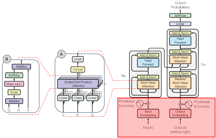
In the overall transformer architecture, this tutorial will cover the blocks highligned in the red box as shown below.

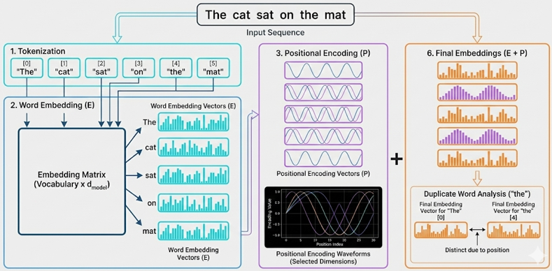
The detailed infographics of this tutorial is as follows.

NOTE : This tutorial uses simplified tokenization (whitespace-based) and random word embeddings for demonstration purposes. Real Transformers use learned embeddings and more sophisticated tokenization (e.g., BPE, WordPiece). The core concept of positional encoding remains the same: using sinusoidal functions to inject position information. The embedding dimension (d_model) is adjustable (16-64) to keep visualizations readable; real Transformers typically use d_model = 512 or higher. The sinusoidal positional encoding formula is: PE_{(pos, 2i)} = sin(pos / 10000^2i/d_model) and PE_{(pos, 2i+1)} = cos(pos / 10000^2i/d_model), where pos is the position and i is the dimension index.

 

Usage Example

Follow these steps to explore how Transformers convert text into numerical embeddings with positional information:

1. Initial State: When you first load the simulation, you'll see the default text "The cat sat on the mat" already processed. The visualization shows seven main components: (1) Tokenization display showing tokens and vocabulary, (2) One-Hot Token Vectors heatmap, (3) Word Embeddings heatmap, (4) Positional Encoding heatmap, (5) Positional Encoding waveforms, (6) Final Embeddings heatmap, and (7) Cosine Similarity Analysis (if duplicate words exist). Notice that the word "the" appears twice at different positions (positions 0 and 4).
2. Observe Tokenization: The first section shows the tokenization results:
   • Tokens are displayed with their position indices (e.g., [0] "The", [1] "cat")
   • The vocabulary shows how each unique word is assigned a token ID (e.g., "The" → ID: 0)
   • This is the first step: text → tokens → token IDs
   This demonstrates how text is converted into discrete tokens and assigned IDs.
3. Observe One-Hot Token Vectors: The second heatmap shows one-hot token vectors:
   • Each token is represented as a sparse binary vector (size = vocab_size)
   • Only the position corresponding to the token's ID is 1, all others are 0
   • Same words have identical one-hot vectors (e.g., both "the" instances have 1 at the same position)
   • You can see the sparse nature - most values are 0 (black), only one is 1 (bright cyan)
   • The visualization uses a simple black/cyan color scheme for binary data (no colorbar needed)
   This demonstrates the intermediate representation between tokens and embeddings.
4. Observe Word Embeddings: The third heatmap shows the Word Embeddings (E) - dense vectors obtained via embedding matrix lookup:
   • Each one-hot vector is multiplied by the embedding matrix to get a d_model-dimensional vector
   • Each token has a d_model-dimensional vector (default: 32 dimensions)
   • The same word at different positions has the same embedding (e.g., both "the" instances have identical rows)
   • Different words have different embeddings
   • You can hover over cells to see exact values
   This demonstrates that word embeddings alone don't contain position information. The embedding lookup transforms sparse one-hot vectors into dense continuous vectors.
5. Observe Positional Encoding: The fourth heatmap shows the Positional Encodings (P) - sinusoidal patterns that encode position information:
   • Each position has a unique encoding pattern
   • The pattern varies smoothly across positions (you can see wave-like patterns)
   • Even dimensions use sine functions, odd dimensions use cosine functions
   • Different dimensions have different frequencies (wavelengths)
   The waveform chart below shows how specific dimensions vary across positions, clearly showing the sine/cosine patterns.
6. Observe Final Embeddings: The sixth heatmap shows the Final Embeddings (E + P) - the sum of word embeddings and positional encodings:
   • This is what actually gets fed into the Transformer
   • Notice that the same word at different positions now has different final embeddings
   • The positional encoding has "shifted" the word embeddings
   This is the key insight: positional encoding makes identical words numerically distinct based on their position.
7. The "the" Test: Scroll down to see the Cosine Similarity Analysis section (if your text contains duplicate words):
   • Word Embedding Similarity: Should be ~1.0 (identical words, identical embeddings)
   • Final Embedding Similarity: Should be < 1.0 (same word, different positions)
   • The difference shows how much positional encoding affects the representation
   This mathematically proves that positional encoding makes position-dependent representations.
8. Experiment with Different Texts: Use the dropdown menu to select from pre-loaded example sentences:
   • Short sentences: "Hello world this is a simple example"
   • Long sentences: "The quick brown fox jumps over the lazy dog"
   • Sentences with repeated words: "Time flies like an arrow fruit flies like a banana"
   • Various patterns to demonstrate different tokenization and embedding behaviors
   Observe how the heatmaps change with different sequence lengths and word patterns. The dropdown provides quick access to example sentences that demonstrate various concepts.
9. Adjust Embedding Dimension: Use the d_model slider to change the embedding dimension (16-64):
   • Lower dimensions (16): Fewer features, simpler patterns, easier to visualize
   • Higher dimensions (64): More features, richer representations, harder to visualize
   • Real Transformers use d_model = 512 or higher, but that's too large to visualize
   Notice how the positional encoding patterns change with different dimensions - more dimensions mean more frequency components.
10. Study the Waveforms: Look at the Positional Encoding Waveforms chart:
    • All dimensions are plotted - every dimension from 0 to d_model-1 is displayed
    • Each dimension has a unique color (distributed evenly across the hue spectrum)
    • Different dimensions show different frequencies (some oscillate faster, some slower)
    • Lower dimensions (e.g., 0, 1, 2) have longer wavelengths (change slowly across positions)
    • Higher dimensions (e.g., 30, 31) have shorter wavelengths (change quickly across positions)
    • The legend shows all dimensions in a compact multi-column layout
    • This creates a unique "signature" for each position
    This demonstrates the physics behind positional encoding - it's literally adding sine and cosine waves of different frequencies. All dimensions are visible to show the complete positional encoding pattern.
11. Understand the Math: The positional encoding formula uses:
    • PE_{(pos, 2i)} = sin(pos / 10000^2i/d_model) for even dimensions
    • PE_{(pos, 2i+1)} = cos(pos / 10000^2i/d_model) for odd dimensions
    • The 10000^2i/d_model term creates different frequencies for different dimensions
    • This ensures each position has a unique encoding pattern
    The combination of sine and cosine at different frequencies creates a rich positional representation.

Tip: The key insight is that Transformers need positional encoding because they process sequences in parallel (unlike RNNs which process sequentially). Without positional encoding, "the" at position 0 and "the" at position 4 would be identical, and the model couldn't distinguish word order. The sinusoidal encoding provides a unique "fingerprint" for each position that can be learned and used by the attention mechanism. Try the default text first to see the "the" test in action, then experiment with your own sentences to see how different patterns affect the embeddings.

Parameters

Followings are short descriptions on each parameter

• Input Text (Dropdown): A dropdown menu with pre-loaded example sentences to demonstrate various concepts. The default selection is "The cat sat on the mat" which contains a duplicate word ("the" at positions 0 and 4) to demonstrate how positional encoding affects identical words at different positions. The dropdown includes sentences of varying lengths and patterns (short, long, with repeated words, etc.) for easy experimentation. The text is tokenized using simple whitespace splitting (in real Transformers, more sophisticated tokenization like BPE or WordPiece is used). Each selection shows how it gets converted through the pipeline: text → tokens → one-hot vectors → embeddings → final embeddings.
• Tokenization: The process of splitting text into tokens (words) and assigning token IDs. This tutorial uses simple whitespace-based tokenization for demonstration. Each unique word in the vocabulary is assigned a unique integer ID (0, 1, 2, ...). The tokenization display shows: (1) All tokens with their position indices [0], [1], [2], etc., and (2) The vocabulary mapping (word → token ID). Real Transformers use sophisticated tokenization methods like Byte Pair Encoding (BPE) or WordPiece, which can split words into subwords and handle out-of-vocabulary words.
• One-Hot Token Vectors: Sparse binary vectors representing tokens in vocabulary space. Each token is represented as a vector of size vocab_size, where only the position corresponding to the token's ID is 1, and all other positions are 0. For example, if "The" has token ID 0 in a vocabulary of 6 words, its one-hot vector is [1, 0, 0, 0, 0, 0]. The one-hot heatmap shows this sparse representation using a simple black/cyan color scheme: black cells represent 0s (most cells), bright cyan cells represent 1s (one per row). Same words have identical one-hot vectors regardless of position. The visualization does not include a colorbar since it's binary data (only 0 or 1). These vectors are the input to the embedding matrix lookup operation.
• Embedding Dimension (d_model): An adjustable slider (range: 16 to 64, default: 32) that controls the size of the embedding vectors. This is the dimension of the embedding space - each token gets represented as a d_model-dimensional vector after embedding lookup. Lower values (16) are easier to visualize but have limited representational capacity. Higher values (64) provide richer representations but are harder to visualize. Real Transformers typically use d_model = 512 or higher, but those are too large to visualize effectively. The slider allows you to experiment with different dimensions and see how it affects both word embeddings and positional encoding patterns.
• Word Embeddings (E): Dense vector representations of tokens obtained via embedding matrix lookup. The embedding matrix has shape [vocab_size, d_model] and transforms one-hot token vectors (size vocab_size) into dense embedding vectors (size d_model). The operation is: One-Hot Vector × Embedding Matrix = Embedding Vector. Each unique word in the vocabulary has a d_model-dimensional embedding vector. In this tutorial, embeddings are randomly initialized (in practice, they are learned during training). The word embedding heatmap shows embeddings for all tokens in the input sequence, with each row representing one token's embedding vector. Identical words have identical embeddings (e.g., both instances of "the" have the same row in the heatmap) because they use the same embedding matrix row.
• Positional Encodings (P): Sinusoidal patterns that encode position information. Each position in the sequence gets a unique d_model-dimensional encoding vector. The encoding uses the formula: PE_{(pos, 2i)} = sin(pos / 10000^2i/d_model) for even dimensions and PE_{(pos, 2i+1)} = cos(pos / 10000^2i/d_model) for odd dimensions. This creates different frequencies for different dimensions, ensuring each position has a unique "fingerprint". The heatmap shows positional encodings for all positions, and the waveform chart shows how specific dimensions vary across positions, clearly visualizing the sine/cosine patterns.
• Final Embeddings (E + P): The sum of word embeddings and positional encodings. This is what actually gets fed into the Transformer layers. The formula is: Final = WordEmbedding + PositionalEncoding. This addition combines semantic information (from word embeddings) with positional information (from positional encodings). The heatmap shows the final embeddings, and you can see that identical words at different positions now have different final embeddings due to the positional encoding component.
• Cosine Similarity: A measure of similarity between two vectors, calculated as the cosine of the angle between them. Values range from -1 (opposite) to 1 (identical). The tutorial calculates cosine similarity between duplicate words to demonstrate: (1) Word embedding similarity (should be ~1.0 for identical words) and (2) Final embedding similarity (should be < 1.0 for the same word at different positions). The difference between these two similarities shows how much positional encoding affects the representation. This provides mathematical proof that positional encoding makes position-dependent representations.
• Tokenization: The process of splitting text into tokens (words). This tutorial uses simple whitespace-based tokenization for demonstration. Real Transformers use more sophisticated methods like Byte Pair Encoding (BPE) or WordPiece, which can split words into subwords and handle out-of-vocabulary words. The tokenized sequence determines the sequence length, which affects the size of the embedding matrices.
• Sequence Length: The number of tokens in the input text. This determines how many rows appear in the heatmaps (one row per token/position). Longer sequences have more positions, and the positional encoding creates unique patterns for each position. The maximum sequence length that Transformers can handle is typically limited (e.g., 512 or 1024 tokens) due to computational constraints.
• Vocabulary: The set of unique tokens (words) in the input text. Each unique token gets assigned an embedding vector. The vocabulary size determines the number of rows in the word embedding matrix. In this tutorial, the vocabulary is built dynamically from the input text. Real Transformers use fixed vocabularies (e.g., 30,000-50,000 tokens) that are determined during training.

Controls and Visualizations

Followings are short descriptions on each control and visualization

• Input Text Dropdown: A dropdown menu with pre-loaded example sentences. The default selection is "The cat sat on the mat" which demonstrates the duplicate word effect (the word "the" appears at positions 0 and 4). Selecting a different sentence from the dropdown automatically updates all visualizations to show the embeddings for the new text. The dropdown includes various examples: short sentences, long sentences, sentences with repeated words, etc. The text is tokenized using whitespace splitting, and each token gets converted into embeddings.
• Embedding Dimension Slider (d_model): An adjustable slider (range: 16 to 64, default: 32) that controls the size of embedding vectors. The current value is displayed next to the slider. Changing the slider immediately recalculates all embeddings and updates all visualizations. Lower dimensions are easier to visualize, higher dimensions provide richer representations. Real Transformers use d_model = 512 or higher, but those are too large to visualize effectively.
• Tokenization Display: Shows the tokenization results in a text format. Displays: (1) All tokens with their position indices [0], [1], [2], etc., and (2) The vocabulary mapping showing how each unique word is assigned a token ID (e.g., "The" → ID: 0). This demonstrates the first step of text processing: text → tokens → token IDs.
• One-Hot Token Vectors Heatmap: A Canvas-based heatmap showing the one-hot token vectors. Each row represents a token's one-hot vector (size = vocab_size), and each column represents a vocabulary position. The color scheme uses black for 0s (most cells) and bright cyan for 1s (one per row), making the sparse nature clearly visible. Only one position per row is 1 (the token's ID position), all others are 0. No colorbar is shown since it's binary data (only 0 or 1). Identical words have identical rows (e.g., both "the" instances show 1 at the same vocabulary position). This demonstrates the sparse intermediate representation between tokens and embeddings. The visualization uses HTML5 Canvas for rendering.
• Word Embeddings Heatmap: A Canvas-based heatmap showing the word embedding matrix (E). Each row represents a token's embedding vector (size = d_model), and each column represents a dimension (labeled 0, 1, 2, ... without "Dim" prefix). The color scale (Red-Blue) shows positive values in red and negative values in blue, with colors near zero appearing as dark blue or dark red. A colorbar on the right shows the value range. Identical words have identical rows (e.g., both "the" instances show the same pattern). This demonstrates that word embeddings alone don't contain position information. The embeddings are obtained via embedding matrix lookup: One-Hot Vector × Embedding Matrix = Embedding Vector. The visualization uses HTML5 Canvas for rendering.
• Positional Encoding Heatmap: A Canvas-based heatmap showing the positional encoding matrix (P). Each row represents a position's encoding vector (size = d_model), and each column represents a dimension (labeled 0, 1, 2, ... without "Dim" prefix). The color scale (Red-Blue) shows the sinusoidal patterns - you can see wave-like patterns across positions. Even dimensions use sine functions, odd dimensions use cosine functions. Each position has a unique pattern, demonstrating how positional encoding creates position-dependent representations. The encoding is independent of the tokens - it only depends on the position. A colorbar on the right shows the value range. The visualization uses HTML5 Canvas for rendering.
• Positional Encoding Waveforms Chart: A Canvas-based line chart showing how all dimensions of the positional encoding vary across positions. Every dimension from 0 to d_model-1 is plotted as a separate line, each with a unique color (distributed evenly across the hue spectrum, creating a rainbow-like appearance). This clearly visualizes the sine/cosine waveforms - you can see how different dimensions have different frequencies (some oscillate slowly, some quickly). Lower dimensions (e.g., 0, 1, 2) have longer wavelengths (change slowly), higher dimensions (e.g., 30, 31) have shorter wavelengths (change quickly). The legend shows all dimensions in a compact multi-column layout. Lines are drawn without markers to avoid clutter when showing all dimensions. This demonstrates the physics behind positional encoding - it's literally adding sine and cosine waves of different frequencies. The visualization uses HTML5 Canvas for rendering.
• Final Embeddings Heatmap: A Canvas-based heatmap showing the final embedding matrix (E + P) - the sum of word embeddings and positional encodings. This is what actually gets fed into the Transformer layers. Each row represents a token's final embedding vector (size = d_model), and each column represents a dimension (labeled 0, 1, 2, ... without "Dim" prefix). Notice that identical words at different positions now have different rows (e.g., "the" at position 0 and "the" at position 4 have different patterns). This demonstrates that positional encoding makes position-dependent representations. The operation is simply: Final Embedding = Word Embedding + Positional Encoding. The color scale (Red-Blue) shows positive values in red and negative values in blue, with a colorbar on the right showing the value range. The visualization uses HTML5 Canvas for rendering.
• Cosine Similarity Analysis: A section that appears when the input text contains duplicate words. It calculates and displays: (1) Word Embedding Similarity - cosine similarity between the raw word embeddings of duplicate words (should be ~1.0 since same word has same embedding), (2) Final Embedding Similarity - cosine similarity between the final embeddings of duplicate words at different positions (should be < 1.0 since positional encoding makes them different), and (3) Difference - showing how much positional encoding affects the representation. This provides mathematical proof that positional encoding makes identical words numerically distinct based on their position. The analysis automatically finds the first duplicate word in the sequence and compares its instances.
• Canvas-Based Visualizations: All visualizations use HTML5 Canvas for rendering, providing fast and efficient rendering of the heatmaps and line charts. The color scales help identify patterns - red indicates positive values, blue indicates negative values, and colors near zero appear as dark blue or dark red. The visualizations update automatically when you change the input text or embedding dimension. Dimension labels show only numbers (0, 1, 2, ...) without the "Dim" prefix for cleaner presentation.

Key Concepts and Implementation

This tutorial demonstrates how Transformers convert text into numerical embeddings with positional information. Here are the key concepts:

• Why Positional Encoding is Needed: Transformers process sequences in parallel (unlike RNNs which process sequentially), so they have no inherent notion of word order. Without positional encoding, "the" at position 0 and "the" at position 4 would be identical to the model. Positional encoding injects position information so the model can distinguish word order. This is crucial for understanding language, where word order matters (e.g., "dog bites man" vs. "man bites dog").
• Sinusoidal Positional Encoding Formula: The standard positional encoding uses sinusoidal functions:
  • Even dimensions (2i): PE_{(pos, 2i)} = sin(pos / 10000^2i/d_model)
  • Odd dimensions (2i+1): PE_{(pos, 2i+1)} = cos(pos / 10000^2i/d_model)
  where pos is the position (0, 1, 2, ...), i is the dimension index (0, 1, 2, ...), and d_model is the embedding dimension. The 10000^2i/d_model term creates different frequencies for different dimensions - lower dimensions have longer wavelengths (change slowly), higher dimensions have shorter wavelengths (change quickly). This creates a unique "fingerprint" for each position.
• Why Sine and Cosine: Using both sine and cosine functions provides several advantages: (1) They create smooth, continuous patterns that can be learned by the model, (2) They allow the model to attend to relative positions (e.g., "position 5 is 3 steps after position 2"), (3) They can extrapolate to longer sequences than seen during training, (4) The combination of different frequencies creates rich positional representations. The alternating pattern (sin for even, cos for odd) ensures each dimension contributes uniquely to the encoding.
• Word Embeddings vs. Positional Encodings: Word embeddings (E) capture semantic meaning - similar words have similar embeddings regardless of position. Positional encodings (P) capture position information - each position has a unique encoding pattern. The final embeddings (E + P) combine both: semantic information from word embeddings and positional information from positional encodings. This addition (not concatenation) allows the model to learn how to use both types of information together.
• The "the" Test: When the same word appears at different positions (e.g., "the" at positions 0 and 4 in "The cat sat on the mat"), the cosine similarity analysis proves that: (1) Word embeddings are identical (similarity ≈ 1.0) - same word, same semantic meaning, (2) Final embeddings are different (similarity < 1.0) - same word, different positions. This mathematical proof demonstrates that positional encoding successfully makes position-dependent representations. The difference between these similarities shows how much positional encoding affects the representation.
• Frequency Patterns: The waveform chart shows all dimensions (0 to d_model-1), each with a unique color, demonstrating how different dimensions have different frequencies. Lower dimensions (e.g., 0, 1, 2) oscillate slowly across positions (long wavelength), while higher dimensions (e.g., 30, 31) oscillate quickly (short wavelength). This creates a hierarchical representation where different frequency components capture different aspects of position. The model can learn to attend to specific frequency components for different tasks. By plotting all dimensions simultaneously, you can see the complete frequency spectrum of positional encoding.
• Embedding Dimension (d_model): The size of embedding vectors affects both word embeddings and positional encodings. Larger dimensions provide richer representations but are harder to visualize. Real Transformers use d_model = 512 or higher, but this tutorial uses 16-64 for visualization. The positional encoding formula scales with d_model - more dimensions mean more frequency components, creating richer positional representations.
• Tokenization: This tutorial uses simple whitespace-based tokenization for demonstration. Real Transformers use sophisticated tokenization methods like Byte Pair Encoding (BPE) or WordPiece, which can: (1) Split words into subwords (e.g., "unhappiness" → ["un", "happiness"]), (2) Handle out-of-vocabulary words, (3) Create fixed-size vocabularies (typically 30,000-50,000 tokens). The tokenization method affects the vocabulary size and how words are represented.
• Learnable vs. Fixed Positional Encoding: This tutorial uses fixed sinusoidal positional encoding (as in the original Transformer paper). Some modern models use learnable positional encodings (embeddings that are learned during training). Fixed encodings have advantages: (1) They can extrapolate to longer sequences, (2) They don't require additional parameters, (3) They provide interpretable frequency patterns. Learnable encodings can adapt to specific tasks but may not generalize to longer sequences.
• What to Look For: When exploring the tutorial, observe: (1) How word embeddings are identical for the same word at different positions, (2) How positional encodings create unique patterns for each position, (3) How final embeddings combine both (same word at different positions now has different embeddings), (4) The waveform patterns showing different frequencies for different dimensions, (5) The cosine similarity analysis proving that positional encoding makes position-dependent representations, (6) How changing d_model affects the richness of positional patterns, (7) How different sequence lengths create different positional encoding patterns. This demonstrates the fundamental mechanism that allows Transformers to process sequences while maintaining awareness of word order.