This interactive tutorial visualizes the Add & Norm (Residual Connections and Layer Normalization) mechanism, which wraps around Attention and FFN modules. Conceptual Link: While previous modules (Attention, FFN) were about *changing* the data, Module 5 ensures we don't lose the original information ("Add") and keeps the numbers mathematically stable ("Norm"). This mechanism provides stabilization and flow control in the Transformer architecture.

The tutorial demonstrates the complete Add & Norm pipeline: Stage A: The Split & Add Operation - A unified visualization showing the input vector splitting into two paths (Identity path preserves original information, Transformation path processes through Attention/FFN), then merging through element-wise addition (x + F(x)), which may produce large/unstable values, and Stage B: The "Norm" Operation (Layer Normalization) - A three-step process that stabilizes the values: Step B1: Calculate Stats (μ, σ) shows the input vector with mean line and displays calculated statistics, Step B2: Normalize (x̂ = (x - μ) / σ) applies centering and scaling to produce a normalized vector, and Step B3: Scale & Shift (y = γ·x̂ + β) applies learnable parameters gamma and beta to produce the final output. The result is a stable, normalized vector ready for the next layer.

The tutorial visualizes the "Highway" metaphor: the Identity path acts as a "highway" that preserves the original signal, while the Transformation path is a "diversion" that processes the data. The Add operation merges both paths, and Layer Normalization ensures the result remains stable even when values become large. This mechanism is crucial for deep networks - without it, gradients can explode or vanish, and original information can be lost through multiple transformations.

In the overall transformer architecture, this tutorial will cover the blocks highligned in the red box as shown below.

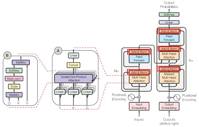
The detailed infographics of this tutorial is as follows.

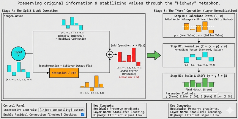
NOTE : This tutorial uses 5D vectors for visualization clarity. Real Transformers use much higher dimensions (typically d_model = 512 or 768). The tutorial demonstrates the Add & Norm mechanism where residual connections preserve information and Layer Normalization stabilizes values. The formula for Layer Normalization is: LayerNorm(x) = γ * (x - μ) / (σ + ε) + β, where μ is the mean, σ is the standard deviation, γ and β are learnable parameters (determined during training), and ε is a small constant. This tutorial breaks down the formula into three steps: (1) Step B1: Calculate statistics (μ and σ) with visual mean line, (2) Step B2: Normalize (x̂ = (x - μ) / σ) to show how centering and scaling work, and (3) Step B3: Scale & Shift (y = γ·x̂ + β) with interactive sliders for gamma and beta. The key insight is that Add & Norm wraps around each sublayer (Attention and FFN), ensuring information flow and numerical stability throughout the deep network.

 

Usage Example

Follow these steps to explore how Add & Norm works:

1. Initial State: When you first load the simulation, you'll see the Add & Norm pipeline with two main stages: (A) The Split & Add Operation (unified schematic showing input splitting into two paths, processing, and addition), and (B) The "Norm" Operation (Layer Normalization with three steps). The visualization shows a single token vector (dimension 5) being processed through the residual connection and normalization mechanism.
2. Stage A: The Split & Add Operation: A unified visualization showing the complete flow from input through split, transformation, and addition in a single schematic diagram:
   • Input Node: A cyan circle labeled "Input" on the left represents the input vector x
   • The Split: The input splits into two parallel paths:
     • Top Path (Identity/Residual): Goes up and straight across, labeled "Identity (Residual)". This path does NOTHING - it just carries the input vector forward unchanged. Color: Cyan (#00FFFF). At the end of this path, a bar chart shows the input vector x values.
     • Bottom Path (Transformation): Goes down and passes through an orange rectangular box labeled "Attention / FFN" (representing Module 3 or Module 4), then continues. The label "Transformation" appears below the box. This path contains the processed vector F(x) from Attention or FFN. Color: Orange (#FF8800). At the end of this path, a bar chart shows the sublayer output F(x) values.
   • The Add Operation: Both paths converge at a green plus sign (+), indicating element-wise addition. The operation x + F(x) merges the preserved original information (from Identity path) with the transformed information (from Transformation path). The result is displayed as a bar chart: Yellow (#FFD700) for stable values, Red (#FF4444) for unstable values (when instability is injected). An arrow (→) points to the next stage.
   • Visual Layout: The entire flow is shown in a single unified canvas (700px × 350px), combining the schematic diagram (lines, boxes, labels) with the actual data (bar charts). This makes it clear that F(x) comes from processing through Attention/FFN, while x bypasses it via the residual connection.
   This unified visualization demonstrates the complete flow: input splits into identity and transformation paths, the transformation path goes through processing, and both paths merge through addition.
3. Stage B: The "Norm" Operation (Layer Normalization): The normalization process stabilizes the values through three steps that visualize the complete LayerNorm formula:
   • Step B1: Calculate Stats (μ, σ): Shows the input vector (result from Stage A addition) with a dashed white line representing the mean (μ). The calculated values are displayed: μ (mean) and σ (standard deviation). This visual representation helps understand "centering" - you can see where the mean lies relative to the bars. Color: Orange (#FF8800) for input vector, White dashed line for mean. The key insight: Even when inputs are huge (after instability injection), you can see the mean line clearly.
   • Step B2: Normalize (x̂ = (x - μ) / σ): Applies the normalization formula: subtract the mean, then divide by standard deviation. This produces a normalized vector where values are centered around 0 and scaled to a healthy range (typically -2 to +2). Visual: The bars are now balanced around zero (some positive, some negative), with a horizontal zero line visible. Color: Cyan (#00FFFF). The magic of normalization: Even if Step B1 shows huge values, Step B2 brings them back to a standard range, preventing explosions!
   • Step B3: Scale & Shift (y = γ·x̂ + β): Applies the learnable parameters gamma (γ) and beta (β) to the normalized vector. Gamma controls "stretch" (scaling) and beta controls "shift" (offset). Interactive sliders allow you to adjust these parameters: Gamma ranges from 0.1 to 3.0 (default 1.0), Beta ranges from -2.0 to 2.0 (default 0.0). Visual: The final output vector, ready for the next layer. Color: Green (#4CAF50). This demonstrates how the network can "undo" normalization if needed by learning specific γ and β values. Note: In real implementations, γ and β are learnable parameters determined during training.
   • The Complete Formula: LayerNorm(x) = γ * (x - μ) / (σ + ε) + β, where μ is the mean, σ is the standard deviation, γ and β are learnable parameters (determined during training), and ε is a small constant (1e-8) to avoid division by zero.
   • Why It Matters: Even if Stage A produces large/unstable values (red bars), Step B2 (Normalize) brings them back to a stable range (cyan bars), and Step B3 (Scale & Shift) applies learnable transformations. This prevents gradient explosions and keeps the network stable while allowing flexibility through learnable parameters.
   This demonstrates the complete normalization process: calculating statistics → normalizing → scaling and shifting with learnable parameters. The step-by-step visualization demystifies Layer Normalization and proves its stabilizing power.
4. Use "Inject Instability" Button: Click this button to simulate a gradient explosion or large sublayer output:
   • Normal State: The sublayer output F(x) has moderate values, and Stage A shows yellow bars (stable) in the Add result
   • After Injection: The sublayer output is multiplied by 10, creating large values
   • Visual Effect in Stage A: The Transformation path bar chart shows huge orange bars, and the Add operation result bars shoot off the chart and turn red (#FF4444), indicating instability
   • Visual Effect in Step B1: The input vector shows huge values, and the mean (μ) and standard deviation (σ) are displayed as very large numbers, clearly showing the instability
   • The Magic Reveal in Step B2: The normalized vector (x̂) looks IDENTICAL to the stable version! This is the key insight: Normalization kills the scale explosion. Even with huge inputs, the normalized output (cyan bars) is in the same healthy range (-2 to +2), proving normalization works.
   • Final Output in Step B3: The final output (green bars) remains stable, ready for the next layer. You can adjust gamma and beta sliders to see how learnable parameters affect the output.
   • This demonstrates why normalization is crucial - without it, large values would propagate and crash the network
   This interactive demonstration proves that Layer Normalization acts as a stabilizer, handling variable scales and preventing numerical explosions. The step-by-step visualization shows exactly how normalization transforms unstable values into stable ones.
5. Use "Toggle Residual" Checkbox: Uncheck this to disable the residual connection:
   • Residual Enabled (Checked): The identity path (cyan) carries the original input forward. The "Add" stage merges original + transformation.
   • Residual Disabled (Unchecked): The identity path becomes zero (all cyan bars disappear). The "Add" stage only contains the transformation, losing the original information.
   • Key Insight: Without residual connections, the original information is lost through multiple transformations. Residual connections preserve the "highway" for information flow.
   This demonstrates why residual connections are necessary: they preserve the original signal, allowing information to flow through deep networks without degradation.
6. Understand the "Highway" Metaphor: The visualization uses a highway metaphor to explain residual connections:
   • The Highway (Top Path): The residual connection is like a highway that bypasses the transformation. It does nothing - just carries the original input forward unchanged.
   • The Diversion (Bottom Path): The sublayer (Attention/FFN) is like a diversion that processes the data. It transforms the input but may lose or modify information.
   • The Merge (Add): Both paths merge, combining the preserved original with the transformation.
   • The Stabilizer (Norm): Layer Normalization ensures the merged result remains stable, regardless of how large the values become.
   This metaphor helps understand that residual connections provide a direct path for information flow, while transformations happen in parallel.
7. Understand Why Add & Norm is Necessary: This mechanism solves two critical problems in deep networks:
   • Problem 1: Information Loss: Through multiple layers, original information can be lost or degraded. Solution: Residual connections preserve the original signal via the identity path.
   • Problem 2: Numerical Instability: Values can grow very large (gradient explosion) or become very small (gradient vanishing). Solution: Layer Normalization centers and scales values to a stable range.
   • Together: Add & Norm wraps around each sublayer (Attention and FFN), ensuring information preservation and numerical stability throughout the deep network.
   This demonstrates that Add & Norm is not just a technical detail - it's essential for training deep Transformers successfully.
8. Observe the Visual Distinction: Notice how the visualization clearly shows stable vs unstable values:
   • Stable Values: Yellow bars in "Add" stage, green bars in "Norm" stage - values are in a healthy range
   • Unstable Values: Red bars in "Add" stage (when instability is injected) - values are too large
   • Normalized Values: Green bars in "Norm" stage - normalization brings unstable values back to a stable range
   • The color coding makes it immediately clear which values are problematic and how normalization fixes them
   This visual distinction helps understand the problem (unstable values) and the solution (normalization) at a glance.

Tip: The key insight is that Add & Norm wraps around each sublayer (Attention and FFN) to provide stabilization and flow control. The "Add" operation preserves original information through residual connections (the "highway"), while "Norm" stabilizes values through Layer Normalization. Use the "Inject Instability" button to see how normalization handles large values - even when the "Add" stage produces red (unstable) bars, the "Norm" stage produces green (stable) bars. Use the "Toggle Residual" checkbox to see what happens without residual connections - the original information is lost. This demonstrates that Add & Norm is essential for deep networks: residual connections preserve information flow, and Layer Normalization prevents numerical explosions. The mechanism ensures that Transformers can be stacked many layers deep while maintaining stability and information preservation.

Description on Stages

This section provides detailed descriptions of each stage in the Add & Norm pipeline:

• Stage A: The Split & Add Operation: This stage uses a unified "schematic + data" visualization to show the complete flow from input through split, transformation, and addition in a single canvas. Visual Elements:
  • Input Node: A cyan circle labeled "Input" on the left (x=30, y=175) represents the input vector x.
  • The Split: The input splits into two parallel paths:
    • Top Path (Identity/Residual): Goes up to y=80 and straight across to the right. Label: "Identity (Residual)". This path does NOTHING - it just carries the input vector x forward unchanged. Color: Cyan (#00FFFF). At the end of this path (x=380), a bar chart shows the input vector x values (5 bars, one per dimension).
    • Bottom Path (Transformation): Goes down to y=270, passes through an orange rectangular box labeled "Attention / FFN" (representing Module 3 or Module 4), then continues. The label "Transformation" appears below the box. This path contains the processed vector F(x) from Attention or FFN. Color: Orange (#FF8800). At the end of this path (x=380), a bar chart shows the sublayer output F(x) values.
  • The Attention/FFN Box: A rectangular box (width: 100px, height: 60px) positioned at x=260 on the bottom path. The box is filled with dark orange (rgba(200, 100, 0, 0.4)) to signify "Processing". It contains the label "Attention / FFN" in gold text, representing the sublayer function F that processes the input.
  • The Add Operation: Both paths converge at a green plus sign (+) positioned at x=580, y=175. The operation x + F(x) merges the preserved original information (from Identity path) with the transformed information (from Transformation path). The result is displayed as a bar chart at x=580: Yellow (#FFD700) for stable values, Red (#FF4444) for unstable values (when instability is injected). An arrow (→) points to the next stage.
  • Visual Layout: The entire flow is shown in a single unified canvas (700px × 350px), combining the schematic diagram (lines, boxes, labels) with the actual data (bar charts). This makes it clear that F(x) comes from processing through Attention/FFN, while x bypasses it via the residual connection. Canvas size: 700×350px.
  • Key Insight: This unified visualization demonstrates the complete flow: input splits into identity and transformation paths, the transformation path goes through processing, and both paths merge through addition. The schematic makes it obvious that the top path (Identity) is a "highway" bypass, while the bottom path (Transformation) goes through the "diversion" of processing.
  Purpose: This stage demonstrates the fundamental concept of residual connections through a unified visualization that combines architecture (schematic) with data (bar charts). The "Highway" metaphor is visually reinforced: one path does nothing (identity), while the other does the work (transformation), and both merge through addition.
• Stage B: The "Norm" Operation (Layer Normalization): This stage shows the complete Layer Normalization formula broken into three steps: Step B1: Calculate Stats (μ, σ), Step B2: Normalize (x̂ = (x - μ) / σ), and Step B3: Scale & Shift (y = γ·x̂ + β). This is the crucial stabilizer that prevents numerical explosions.
  • Step B1: Calculate Stats (μ, σ): Shows the input vector (result from Stage A addition) with visual statistics. The mean (μ) is calculated: μ = (1/n) Σ x[i], and the standard deviation (σ) is calculated: σ = √((1/n) Σ (x[i] - μ)² + ε), where ε is a small constant (1e-8) to avoid division by zero. Visual: The input vector is displayed as vertical bars with a dashed white line representing the mean (μ). The calculated values are displayed above the canvas: μ = [value], σ = [value]. Color: Orange (#FF8800) for input vector, White dashed line (#FFFFFF) for mean line. Canvas size: 200×250px. Key Insight: By seeing the mean line drawn across the bars, users intuitively understand "centering" - the mean shows where the center of the distribution lies. When instability is injected, huge μ and σ values are clearly visible, making the problem obvious.
  • Step B2: Normalize (x̂ = (x - μ) / σ): Applies the normalization formula: first subtract the mean, then divide by standard deviation. Formula: x̂[i] = (x[i] - μ) / σ for each dimension i. This produces a normalized vector where values are centered around 0 and scaled to a healthy range (typically -2 to +2). Visual: The bars are displayed with a horizontal zero line (gray) clearly visible. Bars above zero are positive, bars below zero are negative. The bars are balanced around zero, showing the normalized distribution. Color: Cyan (#00FFFF). Canvas size: 200×250px. The Magic: This is the key insight - even if Step B1 shows huge values (when instability is injected), Step B2 brings them back to a standard range. The normalized vector looks IDENTICAL to the stable version, proving that normalization kills the scale explosion! The zero line makes it clear that values are centered around 0.
  • Step B3: Scale & Shift (y = γ·x̂ + β): Applies the learnable parameters gamma (γ) and beta (β) to the normalized vector. Formula: y[i] = γ * x̂[i] + β for each dimension i. Gamma controls "stretch" (scaling) and beta controls "shift" (offset). Interactive Controls: Two range sliders allow you to adjust these parameters:
    • Gamma (γ) Slider: Range 0.1 to 3.0 (Default 1.0). Controls scaling - values less than 1.0 shrink the normalized vector, values greater than 1.0 stretch it. The current value is displayed next to the slider label. Note: In real implementations, γ is a learnable parameter determined during training (initialized to 1.0).
    • Beta (β) Slider: Range -2.0 to 2.0 (Default 0.0). Controls shifting - negative values shift down, positive values shift up. The current value is displayed next to the slider label. Note: In real implementations, β is a learnable parameter determined during training (initialized to 0.0).
    Visual: The final output vector is displayed with a horizontal zero line (gray). Color: Green (#4CAF50). Canvas size: 200×250px. Key Insight: The sliders allow you to feel how the network retains the ability to "undo" normalization if it needs to, by learning specific γ and β values. This demonstrates that Layer Normalization is not a fixed transformation but can be adapted through learnable parameters that are determined during the training period.
  • The Complete Formula: LayerNorm(x) = γ * (x - μ) / (σ + ε) + β, where μ is the mean, σ is the standard deviation, γ and β are learnable parameters (determined during training), and ε is a small constant (1e-8) to avoid division by zero.
  • Visual Effect: Even if Stage A produces red (unstable) bars with very large values, Step B2 (Normalize) brings them back to cyan (stable) bars in a normal range. Step B3 (Scale & Shift) then applies learnable transformations to produce the final green output. This is the "stabilizer" effect - normalization handles variable scales and prevents numerical explosions, while learnable parameters provide flexibility.
  • Why It Matters: Without normalization, large values from Stage A would propagate through the network, causing gradient explosions and training instability. Normalization ensures values remain in a healthy range regardless of input scale. The step-by-step visualization (stats → normalize → scale & shift) demystifies the black box of Layer Normalization, showing exactly how it transforms the distribution.
  • Layout: The three steps are displayed vertically with downward arrows (↓) between them, showing the sequential flow: Calculate Stats → Normalize → Scale & Shift. Each step has its own canvas and labels, making the progression clear.
  Purpose: This stage demonstrates the complete Layer Normalization process through a three-step visualization that breaks down the formula. The visual transformation from potentially unstable values (red in Stage A) to stable normalized values (cyan in Step B2) to final output (green in Step B3) proves that normalization works as a stabilizer. The step-by-step visualization (calculate stats → normalize → scale & shift) demystifies Layer Normalization, showing exactly how statistics are calculated, how normalization transforms the distribution, and how learnable parameters provide flexibility.

Parameters

Followings are short descriptions on each parameter

• Input Vector (x): The input to the Add & Norm mechanism is a single token vector. Shape: [1, d_model] = [1, 5] in this tutorial (5 dimensions for visualization clarity). Values are generated between -1 and 1. In real Transformers, d_model = 512 or 768. This vector represents the output from a previous layer (e.g., after Attention or FFN). The vector is displayed as a vertical bar chart with 5 bars (one per dimension). Key Concept: This input will split into two paths: the identity path (preserved) and the transformation path (processed).
• Embedding Dimension (d_model): The dimension of input and output vectors (5 in this tutorial for visualization, but 512+ in real Transformers). This is the "standard" dimension used throughout the Transformer. All vectors in the Add & Norm mechanism have this dimension. Shape: [1, d_model] = [1, 5] for a single token vector.
• Sublayer Output (F(x)): The output from a sublayer (Attention or FFN) that processes the input. Shape: [1, d_model] = [1, 5] in this tutorial. This represents the transformed vector after processing by Attention or FFN. Values are generated between -1 and 1 in normal state, but can be multiplied by 10 when instability is injected. The sublayer output is displayed as an orange vertical bar chart (#FF8800). This is the "transformation path" that modifies the input.
• Residual Connection (Identity Path): The path that preserves the original input unchanged. Shape: [1, d_model] = [1, 5] in this tutorial. This path does NOTHING - it just carries the input vector x forward. When enabled, it's identical to the input. When disabled (residual checkbox unchecked), it becomes a zero vector. The residual connection is displayed as a cyan vertical bar chart (#00FFFF). This is the "highway" that bypasses transformation, ensuring original information is always available.
• Add Operation Result (x + F(x)): The result of element-wise addition between the residual connection and sublayer output. Shape: [1, d_model] = [1, 5]. Operation: result[i] = x[i] + F(x)[i] for each dimension i. This intermediate result may contain large/unstable values, especially if the sublayer output is large. Color: Yellow (#FFD700) for stable values, Red (#FF4444) for unstable values (when instability is injected). This is the merged result that combines preserved original information with transformed information.
• Mean (μ): The average of all values in the vector after the Add operation. Calculation: μ = (1/n) Σ x[i], where n is the number of dimensions (5 in this tutorial). The mean is displayed in Step B1 along with a dashed white line drawn across the bars. Subtracting the mean shifts the distribution so the center is at 0, making the vector "zero-centered." When instability is injected, μ becomes very large, clearly showing the problem.
• Standard Deviation (σ): A measure of how spread out the values are. Calculation: σ = √((1/n) Σ (x[i] - μ)² + ε), where ε is a small constant (1e-8) to avoid division by zero. The standard deviation is displayed in Step B1 along with the mean. Dividing by the standard deviation normalizes the scale, bringing values to a healthy range (typically around -2 to +2). When instability is injected, σ becomes very large, clearly showing the problem.
• Normalized Vector (x̂): The result after normalizing: subtract the mean, then divide by standard deviation. Calculation: x̂[i] = (x[i] - μ) / σ for each dimension i. Shape: [1, d_model] = [1, 5]. This is Step B2 of Layer Normalization. The normalized vector has a mean of 0 and a standard deviation of 1, meaning values are in a stable, normalized range. Visual: Displayed with a horizontal zero line (gray), bars above zero are positive, bars below zero are negative. Color: Cyan (#00FFFF). The key insight: Even if Step B1 shows huge values (when instability is injected), Step B2 brings them back to a standard range, proving normalization works!
• Gamma (γ): A learnable parameter that controls scaling (stretch) in Layer Normalization. Range: 0.1 to 3.0 (Default: 1.0). Operation: y[i] = γ * x̂[i] + β for each dimension i. When γ = 1.0, no scaling is applied. When γ < 1.0, the normalized vector is shrunk. When γ > 1.0, the normalized vector is stretched. Gamma allows the network to adjust the scale of normalized values. In real implementations, γ is determined during training (initialized to 1.0). Interactive control: Slider in Step B3 with value display.
• Beta (β): A learnable parameter that controls shifting (offset) in Layer Normalization. Range: -2.0 to 2.0 (Default: 0.0). Operation: y[i] = γ * x̂[i] + β for each dimension i. When β = 0.0, no shift is applied. When β < 0.0, the normalized vector is shifted down. When β > 0.0, the normalized vector is shifted up. Beta allows the network to adjust the offset of normalized values. In real implementations, β is determined during training (initialized to 0.0). Interactive control: Slider in Step B3 with value display.
• Final Output Vector (y): The result after applying gamma and beta to the normalized vector. Calculation: y[i] = γ * x̂[i] + β for each dimension i. Shape: [1, d_model] = [1, 5]. This is Step B3 of Layer Normalization. The final output vector is the result of the complete Layer Normalization process, ready for the next layer. Visual: Displayed with a horizontal zero line (gray). Color: Green (#4CAF50). This demonstrates how learnable parameters (γ and β) allow the network to adapt the normalized values if needed.
• Layer Normalization Formula: The complete Layer Normalization mechanism: LayerNorm(x) = γ * (x - μ) / (σ + ε) + β, where μ is the mean, σ is the standard deviation, γ and β are learnable parameters (determined during training), and ε is a small constant (1e-8). This tutorial breaks the formula into three steps: (1) Step B1: Calculate μ and σ, (2) Step B2: Normalize x̂ = (x - μ) / σ, (3) Step B3: Scale & Shift y = γ·x̂ + β. The step-by-step visualization demystifies Layer Normalization, showing exactly how statistics are calculated, how normalization transforms the distribution, and how learnable parameters provide flexibility.
• Add & Norm Formula: The full Add & Norm mechanism: AddNorm(x, F(x)) = LayerNorm(x + F(x)), where x is the input (residual connection), F(x) is the sublayer output, and LayerNorm is the normalization function. This formula shows the two-step process: (1) Add: x + F(x) merges the preserved original with the transformation, (2) Norm: LayerNorm(·) stabilizes the merged result through centering and scaling. This mechanism wraps around each sublayer (Attention and FFN) in the Transformer.
• Instability Multiplier: When the "Inject Instability" button is clicked, the sublayer output F(x) is multiplied by 10. This simulates a gradient explosion or large sublayer output. The multiplier demonstrates why normalization is necessary - without it, large values would propagate and crash the network. The visualization shows red bars in the "Add" stage (unstable) that are stabilized to green bars in the "Norm" stage (stable), proving that normalization works.

Controls and Visualizations

Followings are short descriptions on each control and visualization

• Inject Instability Button: A button that toggles instability injection. When clicked, the sublayer output F(x) is multiplied by 10, simulating a gradient explosion or large sublayer output. The button text changes to "Reset Stability" when active, and the button turns red. This demonstrates why normalization is necessary - the "Add" stage shows red (unstable) bars, while the "Norm" stage shows green (stable) bars, proving that normalization stabilizes the values.
• Enable Residual Connection Checkbox: A checkbox that toggles the residual connection on/off. When checked (default), the identity path (cyan) carries the original input forward. When unchecked, the identity path becomes zero (all cyan bars disappear), and the "Add" stage only contains the transformation, losing the original information. This demonstrates why residual connections are necessary for preserving information flow.
• Residual Connection Canvas (Stage A - Top Path): Canvas-based vertical bar chart showing the identity path (residual connection). This path does NOTHING - it just carries the input vector x forward unchanged. Color: Cyan (#00FFFF). Label: "Identity (Highway) - Residual Connection". Canvas size: 200×250px. The vector is displayed with 5 bars (one per dimension). This is the "highway" that bypasses transformation, ensuring original information is always available.
• Sublayer Output Canvas (Stage A - Bottom Path): Canvas-based vertical bar chart showing the transformation path (sublayer output F(x)). This path contains the processed vector from Attention or FFN. Color: Orange (#FF8800). Label: "Transformation - Sublayer Output F(x)". Canvas size: 200×250px. The vector is displayed with 5 bars. When instability is injected, values are multiplied by 10, making bars much larger. This is the "diversion" that processes the data.
• Stage A Unified Canvas: A single unified canvas (700px × 350px) that combines schematic diagram and data visualization. The canvas shows: (1) Input node (cyan circle) on the left, (2) Two parallel paths (Identity/Residual top path, Transformation bottom path through Attention/FFN box), (3) Bar charts at the end of each path showing x (cyan) and F(x) (orange), (4) Merging lines converging at a plus sign (+), (5) Add operation result bar chart (yellow/red based on stability), and (6) Arrow pointing to Stage B. This unified visualization makes it clear that F(x) comes from processing through Attention/FFN, while x bypasses it via the residual connection.
• Stats Canvas (Stage B - Step B1): Canvas-based vertical bar chart showing the input vector (result from Stage A addition) with statistics visualization. Color: Orange (#FF8800) for input vector bars, White dashed line (#FFFFFF) for mean line. Canvas size: 200×250px. The visualization shows:
  • The input vector displayed as vertical bars (orange), with bars above zero positive and bars below zero negative
  • A dashed white line drawn horizontally across the bars representing the mean (μ)
  • The mean value (μ) displayed as a label on the mean line
  • A statistics display above the canvas showing calculated values: μ = [value], σ = [value]
  This step visualizes the statistics calculation, making it clear where the mean lies relative to the bars. When instability is injected, huge μ and σ values are clearly visible, making the problem obvious. Value labels are displayed for each bar. The zero line is not shown in this step, but the mean line clearly shows the distribution center.
• Normalized Vector Canvas (Stage B - Step B2): Canvas-based vertical bar chart showing the normalized result after centering and scaling. This is Step B2 of Layer Normalization. Formula: x̂ = (x - μ) / σ. Color: Cyan (#00FFFF). Canvas size: 200×250px. The visualization shows:
  • The normalized vector displayed as vertical bars (cyan), with bars above zero positive and bars below zero negative
  • A horizontal zero line (gray) clearly visible, showing that values are centered around 0
  • Bars balanced around zero, showing the normalized distribution (typically -2 to +2)
  • Value labels displayed showing the normalized values
  This is the key insight: Even if Step B1 shows huge values (when instability is injected), Step B2 brings them back to a standard range. The normalized vector looks IDENTICAL to the stable version, proving that normalization kills the scale explosion! The zero line makes it clear that values are centered around 0.
• Final Output Canvas (Stage B - Step B3): Canvas-based vertical bar chart showing the final output after applying gamma and beta. This is Step B3 of Layer Normalization. Formula: y = γ·x̂ + β. Color: Green (#4CAF50). Canvas size: 200×250px. The visualization shows:
  • The final output vector displayed as vertical bars (green), with bars above zero positive and bars below zero negative
  • A horizontal zero line (gray) clearly visible
  • Value labels displayed showing the final output values
  • Interactive sliders below the canvas allow you to adjust gamma (γ) and beta (β) in real-time
  This demonstrates how learnable parameters (γ and β) allow the network to adapt the normalized values if needed. The sliders let you feel how the network retains the ability to "undo" normalization by learning specific γ and β values. This is the final output of the Add & Norm mechanism, ready for the next layer.
• Gamma (γ) Slider: An interactive range slider for adjusting the gamma parameter in Step B3. Range: 0.1 to 3.0 (Default: 1.0). Step: 0.1. The current value is displayed next to the slider label in yellow. Controls scaling (stretch) of the normalized vector. When γ = 1.0, no scaling is applied. When γ < 1.0, bars shrink. When γ > 1.0, bars stretch. The slider updates the final output canvas in real-time, allowing you to see how gamma affects the output. This demonstrates how the network can learn to adjust the scale of normalized values. Note: In real implementations, γ is a learnable parameter determined during training (initialized to 1.0).
• Beta (β) Slider: An interactive range slider for adjusting the beta parameter in Step B3. Range: -2.0 to 2.0 (Default: 0.0). Step: 0.1. The current value is displayed next to the slider label in yellow. Controls shifting (offset) of the normalized vector. When β = 0.0, no shift is applied. When β < 0.0, bars shift down. When β > 0.0, bars shift up. The slider updates the final output canvas in real-time, allowing you to see how beta affects the output. This demonstrates how the network can learn to adjust the offset of normalized values. Note: In real implementations, β is a learnable parameter determined during training (initialized to 0.0).

Key Concepts and Implementation

This tutorial demonstrates how Add & Norm works, which wraps around Attention and FFN modules to provide stabilization and flow control. Here are the key concepts:

• The Conceptual Link to Previous Modules: Add & Norm serves a different purpose than the transformation modules:
  • Previous Modules (Attention, FFN): These modules *change* the data - they transform representations
  • Module 5 (Add & Norm): This mechanism wraps *around* those modules - it ensures we don't lose original information ("Add") and keeps numbers stable ("Norm")
  • Purpose: Add & Norm provides stabilization and flow control, not transformation
  • This mechanism is applied after each sublayer (Attention and FFN) in the Transformer
  This distinction is crucial - Add & Norm doesn't transform data, it preserves and stabilizes it.
• Add & Norm Architecture: The mechanism consists of two stages:
  • Stage A: The Split & Add - Unified visualization: Input splits into Identity (residual connection) and Transformation (sublayer output) paths, then merges through element-wise addition: x + F(x)
  • Stage B: The Norm - Layer Normalization: Three-step process (Step B1: Calculate Stats, Step B2: Normalize, Step B3: Scale & Shift) with learnable parameters γ and β
  • Full Formula: AddNorm(x, F(x)) = LayerNorm(x + F(x))
  This mechanism wraps around each sublayer, ensuring information preservation and numerical stability.
• Why Residual Connections (The "Add")? Residual connections solve the information loss problem in deep networks:
  • Problem: Through multiple layers, original information can be lost or degraded. Each transformation may modify or discard important information.
  • Solution: The identity path (residual connection) preserves the original signal by carrying it forward unchanged. The "Add" operation merges preserved original (x) with transformation (F(x)).
  • The "Highway" Metaphor: The identity path is like a highway that bypasses transformation, while the sublayer is like a diversion that processes the data. Both paths merge at the "Add" stage.
  • Visual Proof: When you uncheck "Enable Residual Connection", the identity path becomes zero, and the original information is lost. This demonstrates why residual connections are necessary.
  Residual connections ensure that original information is always available, even after multiple transformations.
• Why Layer Normalization (The "Norm")? Layer Normalization solves the numerical instability problem:
  • Problem: Values can grow very large (gradient explosion) or become very small (gradient vanishing) through multiple layers. Large values can cause numerical overflow and training instability.
  • Solution: Layer Normalization centers and scales values to a stable range. Step 1 (Centering) subtracts the mean to center at 0. Step 2 (Scaling) divides by standard deviation to normalize the scale.
  • Visual Proof: When you click "Inject Instability", the "Add" stage shows red (unstable) bars with very large values. The "Norm" stage shows green (stable) bars in a normal range, proving that normalization stabilizes the values.
  • The Math: LayerNorm(x) = (x - μ) / (σ + ε), where μ is the mean, σ is the standard deviation, and ε is a small constant (1e-8) to avoid division by zero.
  Layer Normalization ensures values remain in a healthy range regardless of input scale, preventing numerical explosions.
• The "Highway" Visual Metaphor: The visualization uses a highway metaphor to explain residual connections:
  • The Highway (Top Path - Cyan): The residual connection is like a highway that bypasses the transformation. It does nothing - just carries the original input forward unchanged.
  • The Diversion (Bottom Path - Orange): The sublayer (Attention/FFN) is like a diversion that processes the data. It transforms the input but may lose or modify information.
  • The Merge (Add - Yellow/Red): Both paths merge through element-wise addition, combining preserved original with transformation.
  • The Stabilizer (Norm - Green): Layer Normalization ensures the merged result remains stable, regardless of how large the values become.
  This metaphor helps understand that residual connections provide a direct path for information flow, while transformations happen in parallel.
• Step-by-Step Normalization Math: Layer Normalization is broken down into two clear steps:
  • Step 1: Centering - Calculate mean: μ = (1/n) Σ x[i], then subtract: centered[i] = x[i] - μ. This shifts the distribution so the center is at 0, removing bias.
  • Step 2: Scaling - Calculate std dev: σ = √((1/n) Σ (x[i] - μ)² + ε), then divide: normalized[i] = centered[i] / σ. This normalizes the scale so values are in a healthy range (typically -2 to +2).
  • Result: The normalized vector has mean = 0 and std dev = 1, meaning values are in a stable, standardized range.
  Breaking down normalization into centering and scaling demystifies the black box, showing exactly how it transforms the distribution.
• Why Add & Norm is Essential: This mechanism solves two critical problems in deep networks:
  • Problem 1: Information Loss - Through multiple layers, original information can be lost. Solution: Residual connections preserve the original signal via the identity path.
  • Problem 2: Numerical Instability - Values can grow very large (gradient explosion) or become very small (gradient vanishing). Solution: Layer Normalization centers and scales values to a stable range.
  • Together: Add & Norm wraps around each sublayer (Attention and FFN), ensuring information preservation and numerical stability throughout the deep network.
  Without Add & Norm, deep Transformers would suffer from information degradation and numerical instability, making training impossible.
• Visual Connection to Previous Modules: Add & Norm wraps around the modules we built earlier:
  • After Attention: AddNorm(x, Attention(x)) = LayerNorm(x + Attention(x))
  • After FFN: AddNorm(x, FFN(x)) = LayerNorm(x + FFN(x))
  • Each sublayer (Attention or FFN) is wrapped with Add & Norm to preserve information and stabilize values
  • This allows Transformers to be stacked many layers deep while maintaining stability
  This shows how Add & Norm fits into the larger Transformer architecture, wrapping around each transformation module.
• What to Look For: When exploring the tutorial, observe: (1) How the input splits into two paths (identity and transformation), (2) How the "Add" operation merges both paths, (3) How "Inject Instability" causes red (unstable) bars in "Add" stage, (4) How "Norm" stage stabilizes values to green (stable) bars, (5) How disabling residual connection loses original information, (6) How normalization breaks down into centering (subtract mean) and scaling (divide by std dev). This demonstrates that Add & Norm is essential for deep networks: residual connections preserve information flow, and Layer Normalization prevents numerical explosions.