A radio channel changes the signal on its way to the receiver, and the receiver has to undo that change before it can decode anything. The equalizer is the block that does the undoing. This page starts from what the channel does to the signal, works through the mathematics of reversing it, and finishes with four worked examples.

• What is Equalizer ?
• How it works ?
• Nothing is as easy as said
• Which equalizer should you use ?
• Where does the equalizer sit in a real system ?
• Examples

What is Equalizer ?

Equalization is a process used in communication systems to reverse the distortion incurred by a signal as it travels through a medium (like air in wireless communications)

Equalization acts as a "corrector": An equalizer is a signal processing technique that attempts to reverse these distortions and recover the original data accurately. It's like putting on corrective lenses to see a blurry image clearly.

In wireless communication (actually in any communication), the signal always go through a physical medium (mostly air and anything outside of the transmitter antenna in wirelss communication) before it reaches the reciever. In most cases, these channels tend not to be in the best environement for the signal and put some negative impact on the signal. As a result, the reciever would get the signal that is distorted or corrupted by the channel as illustrated below.

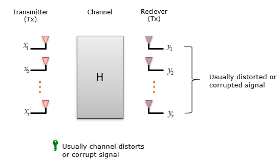
Figure 1. The channel sits between the transmit and the receive antennas and changes the signal on the way through. What arrives at y is a mixture of everything sent from x, scaled and rotated by H.

If the distortion or corruption by the channel gets too serious, proper communication cannot happen. Then, how can we ensure that the transmitted signal(data) can be properly recieved(decoded) by the reciever even when the signal is distorted or corrupted by the wireless channel ? One most common solution is to use a special component called Equalizer. This component can be in the form of hardware or software or both. Equalizer is a special component(a block) that can UNDO the distortion / corruption done by channel while the signal pass through the channel.

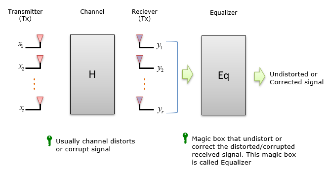
Figure 2. The equalizer is a block after the receive antennas, and its job is to undo H. The drawing calls it a magic box for a good reason: nothing so far says how it learns what H was.

How it works ?

It may sound like a magic when you first heard of what the equalizer do and may ask yourself how such a magic can happen.

To explain on this, I would translate the block diagram shown in previous section into a mathematical format as shown in Figure 3. (If you want to know about further details on H in this equation, refer to channel model page).

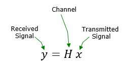
Figure 3. The same picture written as an equation. Every block above becomes one symbol here, and the whole of equalization is the problem of recovering x when only y is known.

As I mentioned above, usally the H distorts or corrupt the signal which make it difficult for the reciever to decode the signal. The goal is to undo the effect of H. Mathematical point of view, it is very simple. Just take the inverse of H (channel) and apply it to the received signal (Hx). Basically what Equalizer do is to calculate the inverse of channel matrix and correct (compensate) the received signal.

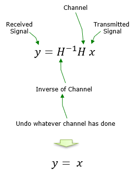
Figure 4. Multiplying by H^-1 cancels H and leaves x. The drawing keeps the name y for the equalizer output, so read the last line as the recovered transmitted signal rather than as the received one.

Let's read that last line carefully, because it hides the whole engineering problem. The receiver multiplies the received vector by H^-1, and H^-1H is the identity matrix, so what comes out is x. That is the entire idea, and on paper it takes one line.

Two things have to be true before the line works, and neither one is free. The receiver has to know H, and H has to be invertible. Everything difficult about equalization sits inside those two conditions.

One more point about the shape of the equation, because the shapes decide the cost. In a MIMO system x is a vector with one entry per transmit layer, y has one entry per receive antenna, and H is the matrix connecting the two. So the inverse the receiver needs is a matrix inverse rather than a scalar division. A 2x2 system needs a 2x2 inverse, a 4x4 system needs a 4x4 one, and the receiver does that work on every symbol it decodes.

• The equalizer applies H^-1 and nothing more exotic : every method on this page answers one question. How do you build that inverse when a plain one does not exist, or would be unwise?
• x, y and H have shapes, and the shapes set the cost : more layers means a bigger matrix to invert, and that inverse is real silicon running at symbol rate.
• The mathematics is one line and the engineering is not : knowing H and being able to invert it are two separate problems. A real receiver has to solve both before this line means anything.

Nothing is as easy as said

As everybody in the engineering would know, there is nothing as easy as said. Same applies to Equalization as well. As mentioned in previous section, ideally Equalization is just to take the inverse of channel matrix and applies it to the received signal, but there are some mathematical and technical chalenges and preconditions.

To obtain the inverse of the channel matrix, the channel matrix should satisfy specific conditions as follows.

• The channel matrix should be square matrix. It means that the number of Tx and Rx antenna should be same. But in reality, there are cases where Tx and Rx antenna are not same.
• The channel matrix should be invertable. It means the matrix should not be 0. 'A matrix is 0' mean 'it's determinant is 0'.

To overcome these mathmatical restriction, we use many other techniques that can applies to non square matrix.  Most of the commonly used Equalization method like least squre, SVD, MMSE can be applied to non-square matrices.

Now let's suppose we have the means to overcome the mathematical constrains. But we still have some practical challenges to overcome.

Conceptually, Equalization is to get the inverse (or pseudo inverse) of the channel matrix. It mean that the channel matrix should be given to Equalizer. How do I (meaning the reciever) know about the channel matrix ? If channel does not change at all, we may investigate about the channel before we build the communication system and preprogram the channel matrix directly into the reciever, but we cannot expect this kind of constant (never changing) channel condition in wireless communication. Channel property changes all the time in wireless environment. It means the reciever itself has to figure out the channel characteristics and build the channel matrix dynamically. This process (i.e, finding out channel characteristics) is called channel estimation. There are various kind of channel estimation techniques and some of those techniques are explained in this page.

Which equalizer should you use ?

The page has been saying 'take the inverse' as though only one way existed. In practice there are several, they give different answers on the same channel, and the difference shows up most on a weak channel. Let's look first at why a plain inverse is a bad idea once there is noise, and then at what each of the four methods does about it.

Start with what the received signal really is. The channel does not only multiply x by H, it also adds noise, so the receiver holds y = Hx + n. Apply H^-1 to all of that and the result is x + H^-1n. The wanted signal comes back exactly. The noise does not, because the equalizer multiplies the noise by H^-1 as well.

That second term is the problem. A weak channel direction has a small singular value, so the inverse scales that direction up by a large factor. It scales the noise sitting in that direction up by the same factor. Engineers call this noise enhancement. It is the reason a perfect inverse is not the best receiver, and it is the reason MMSE exists at all.

The four methods below answer the same question with different amounts of caution. Read the fourth column first, because what each method optimises is what really separates them.

Two of those rows are closer than they look. When H is square and invertible, the zero forcing expression (H^HH)^-1H^H collapses to H^-1, and the two methods produce exactly the same matrix. Figure 6 and Figure 7 are the proof. Both run on the same channel, and both print the same equalizing matrix, with 1 and -j along the top row and 1 and j along the bottom. Zero forcing is worth having on a channel that is not square, where a direct inverse does not exist at all.

SVD is the one that changes the transmitter. The other three run entirely inside the receiver. SVD splits the work across both ends instead. The transmitter multiplies by v before sending, and the receiver multiplies by s^-1u^H after receiving. That buys a set of parallel channels with no interference between them, and it costs a feedback path so the transmitter can learn v. Figure 8 carries an extra Precoded Tx column that none of the other examples has.

MMSE is the practical default in a real receiver. It adds N₀, an estimate of the noise level, to the matrix before inverting it. That addition stops the inverse from growing without limit on a weak direction. As N₀ falls towards zero the expression turns back into the zero forcing one. So MMSE behaves like zero forcing on a clean channel, and better than it on a noisy one.

• Inverting the channel also inverts the noise : the equalizer cannot tell signal from noise. It applies one gain to a weak direction, and that gain reaches the signal and the noise alike.
• Zero forcing and a direct inverse agree on a square channel : the pseudo-inverse is worth the extra algebra only when the matrix is not square, which is the usual case once the antenna counts differ.
• SVD is the only one that needs the transmitter to cooperate : it delivers clean parallel streams and it cannot be a receiver-only decision, so it costs signalling that the other three do not.
• MMSE trades a little interference for much less noise : it does not null the interference between layers completely, and that is the point. The residual interference costs less than the noise that zero forcing would have amplified.

Where does the equalizer sit in a real system ?

So far H has been one matrix for the whole signal, which is a useful picture and not what a real receiver holds. A wideband channel behaves differently at different frequencies, and that is exactly the problem OFDM was designed around. Let's see what the equalizer turns into once OFDM has done its work.

A wideband signal on a multipath channel suffers inter-symbol interference, because echoes of one symbol arrive while the next symbol is still being received. Equalizing that in the time domain needs a filter with many taps, and the number of taps grows with the delay spread. This was genuinely hard work in GSM, and it is why a GSM receiver carried a Viterbi equalizer.

OFDM changes the shape of the problem rather than solving it directly. It splits the band into many narrow subcarriers, and each subcarrier is narrow enough that the channel across it is flat. A flat channel is one complex number, not a filter. So the equalizer for a single antenna OFDM system is one complex division per subcarrier, and nothing more than that.

MIMO puts the matrix back, but only per subcarrier. On each subcarrier the receiver holds a small matrix, two by two for two layers, and it applies one of the methods above to that matrix. The matrices are small and there are a great many of them, which is exactly the shape a hardware pipeline handles well.

Figure 5 puts the equalizer where it actually runs. Notice that it sits after the FFT, and that the channel estimate feeding it comes from the same FFT output rather than from anywhere else.

Figure 5. The equalizer runs after the FFT, on one subcarrier at a time. The channel estimate it needs comes from pilot symbols carried in the same OFDM symbols, which is why channel estimation and equalization are always discussed together.

• OFDM turns a filter into a division : the hard time domain equalizer of a single carrier system becomes one complex number per subcarrier. That is a large part of why OFDM was adopted so widely.
• The matrix comes back with MIMO, one per subcarrier : the size is set by the number of layers rather than by the delay spread, so it stays small however long the echoes are.
• The equalizer cannot run before the channel estimator : both read the same FFT output, and the estimate has to be ready first. A bad channel estimate looks exactly like a bad equalizer from the outside.

Examples

NOTE : Click on the image and it will lead you to the page with more examples and the Octave source code that I wrote for the examples.

All four examples run on the same channel, so you can compare them directly. H is the 2x2 matrix printed at the top of each picture, there are two transmit layers, and the constellation is QPSK. Each picture reads left to right: the transmitted layers first, then what the receive antennas actually see, then the equalized result. The middle column is the one to study hardest, because that is the problem the equalizer has to solve.

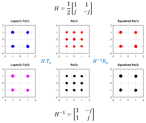
Figure 6. Direct inverse. The matrix printed underneath is H^-1 itself, and the Rx columns show the nine point cloud that two overlapping QPSK layers produce before any equalization.

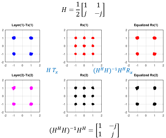
Figure 7. Zero forcing, written here as least square. The expression is the pseudo-inverse (H^HH)^-1H^H, and because this particular H is square and invertible it evaluates to the same matrix as Figure 6.

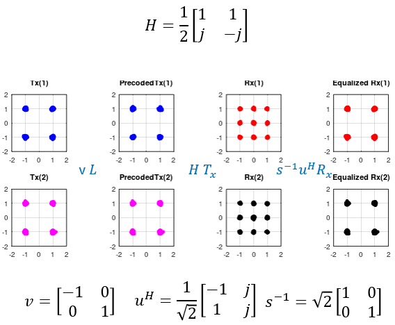
Figure 8. SVD. This example has a Precoded Tx column that the others do not, because the transmitter multiplies by v before sending. The receiver then applies s^-1u^H and the two layers come back separated.

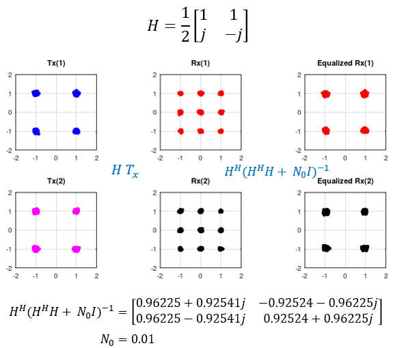
Figure 9. MMSE, run with the noise level set to N₀ = 0.01. The equalizing matrix now depends on that noise estimate, and that dependence is the only thing separating it from the three methods above.

• The same channel in all four : H does not change between the examples, so every difference you see in the right hand column comes from the method rather than from the channel.
• The middle column is the problem statement : two QPSK layers arriving together make a nine point cloud, and no decision rule can recover either layer from that cloud alone.
• Only the SVD example touches the transmitter : its extra column is not decoration. It is the precoding step, and it is what the other three methods manage without.
• Each picture links to its Octave source : the code is worth reading next to the maths, because it shows how few lines each of these methods actually takes.