As everybody knows, 5G/NR is very complicated technology. In learning any kind of complicated topics, usually we take approaches in two different directions. Simply put, one is top-down and the other one is bottom-up. In other words, one is from the details to big picture and the other one is from the big picture to the details.  Which way to take would be up to person and even for the same person the approach would vary depending on the specific topics. Whichever approach you take, you should get both big picture and the details eventually.

This note is to show an example of my own big picture on how 5G/NR PHY layer are configured in terms of parameter settings.

You may or may not agree with this picture. If you agree, take a little bit of closer look at this structure. If you don't, it is completely OK. However, I strongly suggest you to try to draw your own big picture if you don't agree with my flow diagram. Even if yours may be completely different from mine, it will definitely help with understanding NR details.

• How does DCI get the parameter values ?
• Why does DCI carry an index instead of the value ?
• Reference

How does DCI get the parameter values ?

My view on NR physical layer parameter structure is as shown below. The configuration of physical layer at each and every slot at baseband point of view is done by DCI. It means the direct interface to physical layer is DCI, but the DCI interacts with various higher layer components depending on cases. Depending on how DCI interact (is correlated) with higher layer component, I classify them into several cases as shown below.

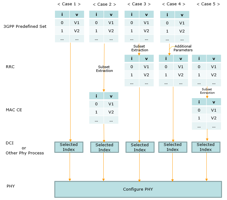
Figure 1. Read it column by column rather than row by row. Every column ends in the same place, and what differs is how many layers the set passes through before DCI picks one entry from it.

• The five rows are labelled 3GPP Predefined Set, RRC, MAC CE, DCI or Other Phy Process, and PHY.
• Each small table drawn in a column has two columns of its own, headed i and v, with rows 0, 1 and an ellipsis.
• Case 1 has a table at the 3GPP Predefined Set row only, and the arrow runs straight down past RRC and MAC CE to Selected Index.
• Case 2 has a table at the 3GPP row and another at the MAC CE row, joined by an arrow labelled Subset Extraction. The RRC row is empty.
• Case 3 has the same shape as Case 2 with the second table at the RRC row instead, and the MAC CE row empty.
• Case 4 also puts its second table at the RRC row, and a curved annotation labelled Additional Parameters feeds into it.
• Case 5 has no table at the 3GPP Predefined Set row at all. Its first table is at RRC, an arrow labelled Subset Extraction leads to a table at MAC CE, and that feeds Selected Index.
• Every column ends at a Selected Index box on the DCI row, and every Selected Index box points down into the single Configure PHY bar.

< Case 1 > is the case where a lot of detailed configuration is defined in the form of big tables in 3GPP documents and DCI points to a specific index value of the table. In this case, it would seem that higher layer (RRC, MAC CE) does not directly (explicitely) get involved in the contents of DCI.  Most case of LTE PHY configuration would belong to this case. In NR, Antenna Port (SISO, MIMO configuration) would belong to this category. To be very specific, in NR antenna port case, RRC is implicitely(indirectly) involved in this process via DMRS configuration, but from high level point of view I think I can categorize it into this case.

< Case 2 > is the case where a wide range of tables are specified in 3GPP specification and a subset of those tables are listed in MAC CE and then DCI select a specific index from MAC CE for each slot configuration.

< Case 3 > is the case where a wide range of tables are specified in 3GPP specification and a subset of those tables are listed in RRC and then DCI select a specific index from RRC for each slot configuration. I think CSI PMI and codebook setting can be categorized into this category. Wide varieties of PMI tables are defined in 3GPP specification as summarizied here, and RRC specifies a subset of tables in ASN as shown here. Another example would CSI RS configuration. In this example, 3GPP specification defines a big table as shown here and RRC select a specific row from the table as shown here, and physical layer process generate CSI RS as RRC specifies.

< Case 4 > is the case where a table(s) is defined in 3GPP and RRC extract a subset from this table and put them togather with some additional parameters as a new table. One famous example for this case is pdsch-TimeDomainAllocation, pusch-TimeDomainAllocation. In this example, 3GPP specification defines a table for SLIV and RRC creates a new table called pdsch-TimeDomainAllocation, pusch-TimeDomainAllocation which is made up of a subset of SLIV table and additional parameters (i.e, K0, K2) as shown here.

< Case 5 > is the case where no 3GPP predefined table sits at the top at all. RRC defines the whole set itself, MAC CE activates a subset of it, and DCI then selects one entry from what MAC CE left active. This is the only column in the diagram whose first table is at the RRC row, and it is the one case the four descriptions above do not cover.

The TCI state flow is the clearest example. PDSCH-Config carries tci-StatesToAddModList, and maxNrofTCI-States is 128, so RRC can define up to 128 states. The TCI States Activation/Deactivation for UE-specific PDSCH MAC CE then sets a T bit per state, and 38.321 puts the maximum number of activated states at 8. DCI reads the Transmission Configuration Indication field, whose codepoint is the ordinal position of a state among those the MAC CE activated.

That last detail is the part worth remembering. The codepoint DCI carries is not the TCI-StateId. 38.321 says the first activated state maps to codepoint 0, the second to codepoint 1, and so on. The same codepoint therefore means a different state after the MAC CE changes. A trace read without the MAC CE beside it cannot be decoded.

The five columns differ on three questions only, and setting them out together is quicker than reading five paragraphs. The first question is where the full set of values is defined. The second is who narrows that set. The third is who picks one entry for a given transmission.

Two patterns follow from the table. The last column is DCI in every case, which is the point the paragraph above the diagram makes about DCI being the direct interface to the physical layer. The middle column is what actually varies, and it is what decides how quickly a value can change. A set narrowed by RRC changes at reconfiguration speed, and a set narrowed by MAC CE changes far faster than that.

• DCI always makes the final choice : every column of the diagram ends at a Selected Index box, so the difference between cases is never about who picks.
• The narrowing step sets the timescale : RRC narrowing changes with reconfiguration, MAC CE narrowing changes with a control element, and Case 1 has no narrowing at all.
• Case 5 starts at RRC : it is the only case with no 3GPP predefined table above it, and TCI states are the example.
• An index is meaningless on its own : except in Case 1, the value DCI carries is an offset into a set that some other layer chose.

Why does DCI carry an index instead of the value ?

The five cases above describe what the structure is. They do not say why it exists, and that is the question worth asking. A reader meeting Figure 1 for the first time usually wonders why the network does not simply put the parameter value into the DCI and leave it there. The answer is a constraint that is easy to state and easy to forget.

DCI is carried on PDCCH. The UE does not know in advance where its DCI is, so it decodes candidate locations blindly, many times per slot. It has to do so at the edge of the cell, where the signal is weakest. Every bit added to a DCI format costs coding room and therefore costs coverage. DCI is the most expensive place in the whole system to put a bit, and the entire structure in Figure 1 exists to keep that field narrow.

The DCI field width sets the size of every set above it

This is the part that turns the diagram from a taxonomy into a design rule, and it is the single most useful idea on this page. The constants that appear in the RRC and MAC specifications are not arbitrary. They are the width of the DCI field that indexes them.

Take the Case 5 example. 38.331 sets maxNrofTCI-States to 128, so RRC may define 128 states. 38.321 caps the activation command at 8 states. 38.212 gives the Transmission Configuration Indication field in DCI format 1_1 as 3 bits when it is present. Two to the power of three is eight. The MAC CE limit is not a MAC decision at all. It is the DCI field width restated.

Figure 2. The narrowing is not arbitrary at any step. 128 is what RRC may define, 8 is what the 3 bit DCI field can address, and the MAC CE exists to decide which 8 of the 128 are reachable right now.

• RRC configures the full list through tci-StatesToAddModList, bounded by maxNrofTCI-States at 128.
• The activation MAC CE sets one bit per state, and 38.321 puts the maximum number of activated states at 8.
• The DCI Transmission Configuration Indication field is 3 bits in format 1_1, which addresses exactly 8 codepoints.
• The codepoint is the ordinal position among the activated states, so codepoint 0 is the first state with its bit set, not TCI-StateId 0.

The same arithmetic appears in Case 4. 38.212 gives the Time domain resource assignment field as 4 bits, and 38.331 sets both maxNrofDL-Allocations and maxNrofUL-Allocations to 16. Two to the power of four is sixteen. Once this pattern is visible, a great many constants in the RRC specification stop looking like magic numbers.

Which layer should hold a parameter, and what moving it costs

The five cases are really five points on one axis, which is how fast a value needs to change. Reading the diagram that way turns it into something usable when a new parameter has to be placed rather than merely looked up.

A 3GPP predefined table never changes, because it is fixed when the specification is frozen. RRC changes at reconfiguration, which costs signalling and can interrupt the connection. A MAC control element changes without any reconfiguration, so it is far cheaper and far faster. DCI changes for every scheduled transmission. The working rule is to place a parameter at the slowest layer that can still track how quickly it has to move, because every layer downward costs more of a scarcer resource.

One consequence of that layering surprises people, and it is worth knowing in advance. An activation command does not take effect when the UE receives it. 38.214 defines the application time relative to the HARQ-ACK the UE sends for the PDSCH that carried the command, not relative to the command itself. There is therefore a window in which the gNB has decided on a new mapping and the UE is still using the old one.

That window is the source of a whole class of intermittent faults. During it, the same DCI codepoint resolves to one state at the gNB and a different state at the UE. Nothing in the DCI looks wrong, and the symptom appears further downstream as a throughput drop or a beam that points the wrong way. When a log shows behaviour like that around a reconfiguration or an activation, the mapping timing is the first thing to check.

• The DCI field width is the real constraint : the set a slower layer may hand down is bounded by two to the power of the field width that indexes it.
• The RRC constants are derived, not chosen : maxNrofDL-Allocations is 16 because the field is 4 bits, and the MAC CE cap is 8 because the field is 3 bits.
• Place a parameter at the slowest layer that can track it : every step down the diagram gains speed and consumes a scarcer resource.
• Activation is not instant : the new mapping applies from a slot referenced to the HARQ-ACK for the activation command, so a window exists where the two ends disagree.
• Never read a DCI field alone : a codepoint is an offset into a set, so the RRC configuration and the MAC CE state at that instant are part of the reading.

Reference

[1] 3GPP TS 38.331 - NR; Radio Resource Control (RRC) protocol specification. PDSCH-Config and tci-StatesToAddModList for the Case 5 example.

[2] 3GPP TS 38.321 - NR; Medium Access Control (MAC) protocol specification. Clause 6.1.3.14 for the TCI States Activation/Deactivation MAC CE.

[3] 3GPP TS 38.212 - NR; Multiplexing and channel coding. The DCI formats that carry the selected index in every case above.