ULA is the Object that is for design and simulating the set of antenna placed along a line. This is the type of array antenna that are used for MIMO (e.g, LTE MIMO).

• Basic Numerical Test
• Plotting Radiation Pattern in 2D
• Plotting Radiation Pattern in 3D
• Steering with Custom Steering Vector
• Example 01
• Disclaimer ! :

Basic Numerical Test

This first script plots nothing. It prints numbers, and the point is to see what a steering vector actually is before it turns into a picture. Every pattern further down this page comes from the two arrays printed here, txmipos and wt.

Four numbers in that output are worth reading before moving on.

The carrier is 26 GHz, so lambda is 11.54 mm and the element spacing lambda/2 is 5.77 mm. That is the 0.0058 the object prints. The txmipos array then divides the element positions by lambda, which is why the middle row reads -0.75, -0.25, 0.25, 0.75: four elements, half a wavelength apart, centred on the origin. The other two rows are zero because the object reports ArrayAxis: 'y', so the array lies along y and nowhere else.

wt is the weight vector. With txang set to broadside every element gets the same weight, which is why wt prints as 1 1 1 1 with no phase at all. The txsv vector points at the angle being tested, and txbeam is the inner product of the two.

That inner product is the whole beamformer in one line. At txbeam_ang = 0 every term adds in phase and txbeam prints 4, which is simply the element count. At txbeam_ang = 10 the terms no longer align and txbeam prints 3.2930, or 0.823 once divided by 4. Note that the plots further down normalise the peak to 1, while this numerical test leaves it unnormalised at N.

• txbeam peaks at N, not at 1 : a coherent sum of N unit weights gives N, and the plotting scripts divide that back out.
• Broadside costs no phase : wt is real and uniform, so a beam pointed at 0 degrees needs no phase shifter setting at all.
• Taper: 1 matters later : the weights are uniform in amplitude throughout this page, and that fixes the sidelobe level.

Plotting Radiation Pattern in 2D

The numbers become a picture here. The script sweeps txbeam_ang across the full -90 to +90 range and plots the magnitude twice, once as a Cartesian curve and once as a polar plot. What changes between the runs is only NoOfTxAntenna and txang.

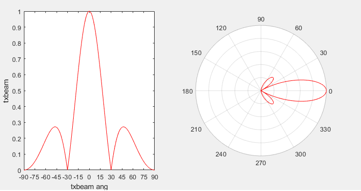
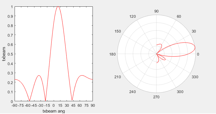
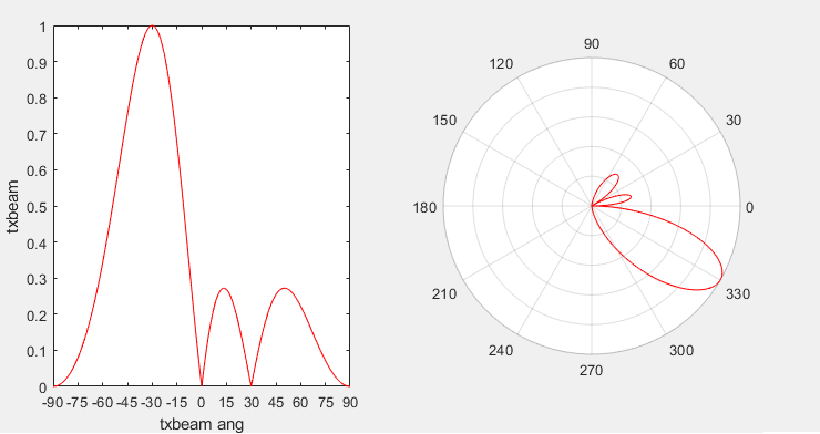
Following three example shows the beam pattern of the array antenna with 4 elements depending on different steering angles.

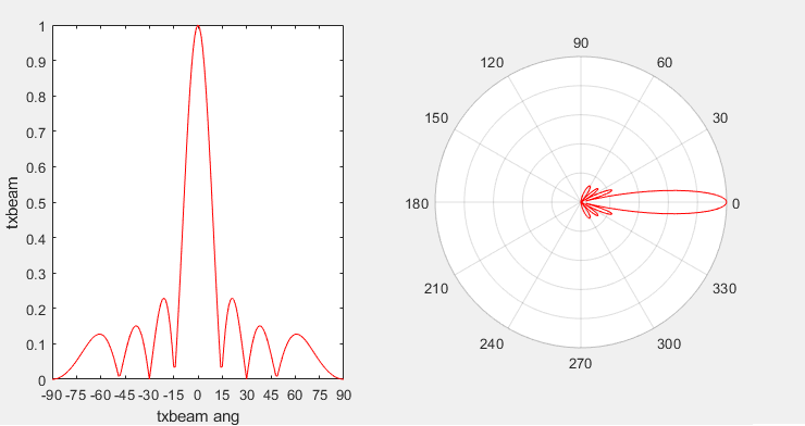
Following three example shows the beam pattern of the array antenna with 8 elements depending on different steering angles.

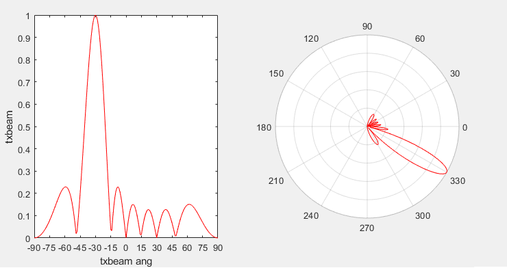
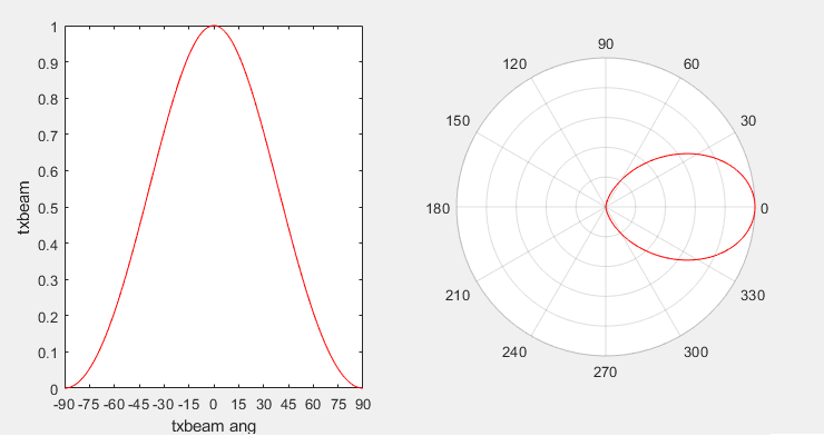
Following three example shows how the shape of the beam changes as the number of antenna elements in an array antenna gets larger.

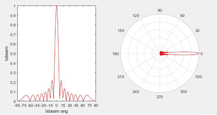
Four element counts appear in this section, and setting their numbers side by side is what makes the plots worth reading. The table below is computed for the same half wavelength ULA the script builds.

Three things follow from that table, and all three are visible in the plots.

Doubling the element count halves the beamwidth. It runs 60 degrees at two elements, 26 at four, 13 at eight and 6 at sixteen. The usual approximation for a half wavelength array is 0.886 lambda / (N d) radians, and it lands within a degree from four elements upward. At two elements it is out by nine degrees, so do not lean on it for very small arrays.

The first null closes in with the beam. It sits where sin(theta) = 2/N, which puts it at 30 degrees for four elements and 7.2 degrees for sixteen. Those are exactly the zero crossings the Cartesian plots show.

The sidelobe level barely moves. It settles near 0.22 in amplitude however many elements are added, which is about -13 dB in power. Adding elements buys angular resolution, and it does not buy a cleaner pattern. Only tapering the element amplitudes does that, and every array on this page runs with Taper: 1.

The runs with txang away from zero show the other half of the story. Steering does not move the beam rigidly, it widens it. For four elements the half power beamwidth is 26.3 degrees at broadside, 30.9 degrees steered to 30 degrees, and 40.6 degrees steered to 45 degrees. The pattern also stops being symmetric about its own main lobe, which the +10 degree run shows plainly.

• Element count sets resolution : each doubling of N halves the beamwidth and halves the angle to the first null.
• Element count does not set sidelobe level : that stays near -13 dB, and only a non-uniform taper changes it.
• Steering costs beamwidth : a beam pushed to 45 degrees is about half as sharp as the same beam at broadside.

Plotting Radiation Pattern in 3D

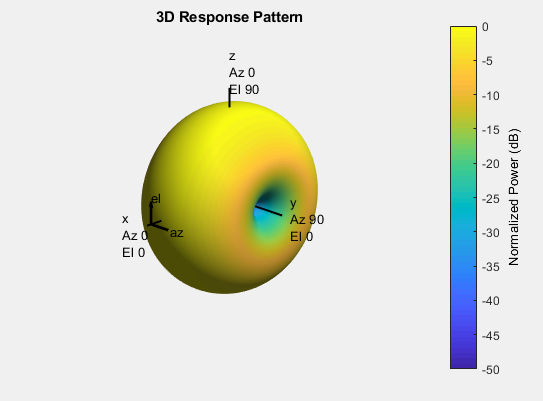
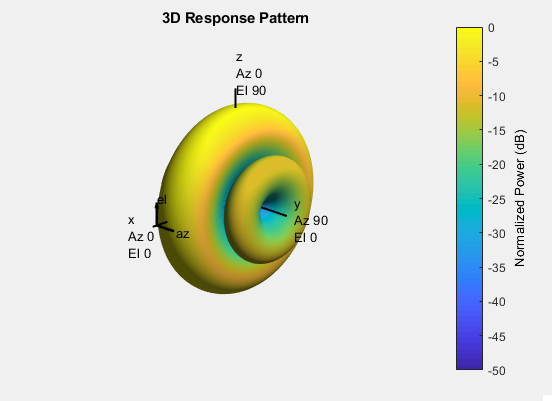
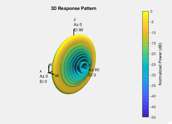
The Cartesian and polar plots cut through the pattern along one plane. These surfaces show what that cut was taken from, and they answer a question the 2D view cannot: what the beam is doing in all the directions the sweep never visited.

All four surfaces share one property, and it is the most useful thing on this page.

They are rotationally symmetric about the y axis. The reason is printed in the very first code output: the object reports ArrayAxis: 'y'. The elements lie along a line, so the array can only tell directions apart by their angle from that line. Every direction at the same angle from y looks identical to it.

So the beam of a ULA is not a pencil. It is a cone, and at large element counts a thin disc. Watch the four surfaces in order and the shape flattens rather than closing up. At two elements it is nearly a sphere with a shallow dimple. At sixteen it is a thin disc ringed with sidelobes, and the hole along y has become a deep well. What never happens is the beam narrowing into a spot.

That is the practical limit of a linear array, and it is why a real base station panel is a planar array rather than a line of elements. Narrowing the beam in two planes at once takes elements in two dimensions.

• A ULA discriminates in one angle only : the pattern is a surface of revolution about the array axis.
• More elements flatten the disc : they do not turn it into a pencil beam.
• The colour scale is normalised power in dB : it runs from 0 at the peak down to -50, so the rings are sidelobes and the dark well along y is the null.

Steering with Custom Steering Vector

Everything so far let phased.SteeringVector build the weights from an angle. This section sets the weights by hand instead, which is how a pattern is produced that no single steering angle would give.

Followings are the examples that we define our own steering vector.

Example 01 >

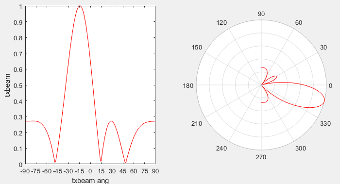
The steering vector in this example (marked red) came from a CSI codebook for NR. It is derived as explained here.

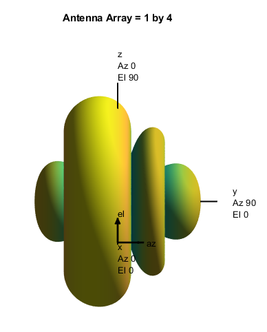
The two plots in this section are worth comparing against the broadside runs earlier, because both differ from anything a single steering angle produces.

In the Cartesian plot the main lobe peaks near -15 degrees, and the two nulls around it are not evenly spaced: one sits near -45 degrees and the other near +15 degrees. The response also climbs again toward both ends of the sweep, so a signal arriving near +90 or -90 degrees is not rejected.

The 3D plot is drawn differently from the earlier surfaces. It is titled Antenna Array = 1 by 4 and carries no dB colour bar, so the main lobe and the sidelobes render as separate solid shapes rather than as one shaded surface. The array is still four elements in a line, and the pattern is still symmetric about the array axis.

The reason to set weights by hand is that you are no longer restricted to the shapes one steering angle can make. Beamwidth, sidelobe level and null position stop being fixed by N alone and become things you choose, at the cost of working out the weights yourself.

• Hand set weights break the symmetry : the nulls no longer sit at equal angles either side of the main lobe.
• The array axis still rules : custom weights change the pattern within the plane, and they cannot give a linear array a pencil beam.
• Check the sweep ends : this pattern rises again near plus and minus 90 degrees, which a steered uniform beam of the same size does not do as strongly.

Disclaimer ! :

This page is only to show you the overall logics and visualization for various Phase Array Antenna System. I haven't investigated much about verifying about the accuracy.

If you think the code is not so efficient, it is 100% my fault. I haven't made any effort for effiecient code. I just tried to create code as simple as possible for the readers. As you know, easy-to-read code is not always efficient for a specific chipset.

If you find any mistake in terms of accuracy, it is also very highly likely be my fault. Not the problem of Matlab tool box itself.

Any comment and corrections if you find any mistake will be welcome and appreciated.