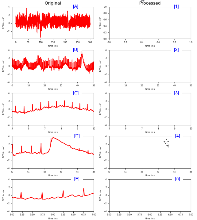
import numpy as np

import matplotlib.pyplot as plt

import scipy as sp

import scipy.misc as spm

from scipy.fftpack import fft

from scipy import signal

################################################################

#                                                        Data Set                                                        #   

################################################################

fs = 360;

fn = fs / 2; # Nyquist Frequency

x = spm.electrocardiogram();

t = np.linspace(0,x.size-1,x.size) / fs;

f = np.linspace(0,x.size-1,x.size) * (fs / x.size);

################################################################

#                                                        PROCESSING                                                    #   

################################################################

n = 101;

a = 1;

ftap = signal.firwin(n,cutoff = 0.15, window = "hamming");

xf = signal.lfilter(ftap, a, x);

################################################################

#                                                        PLOT                                                              #   

################################################################

FontSize_Xlabel = 6;

FontSize_Ylabel = 6;

bw = 0.40;

bh = 0.145;

bx = 0.025;

by = 0.1;

bx_gap = 0.075;

by_gap = 0.05;

by_shift = -0.05;

bx_shift = 0.05;

pltRegion1 = [bx + 0 * (bw + bx_gap) + bx_shift,by + 4*(by_gap + bh) + by_shift, bw, bh];

pltRegion2 = [bx + 0 * (bw + bx_gap) + bx_shift,by + 3*(by_gap + bh) + by_shift, bw, bh];

pltRegion3 = [bx + 0 * (bw + bx_gap) + bx_shift,by + 2*(by_gap + bh) + by_shift, bw, bh];

pltRegion4 = [bx + 0 * (bw + bx_gap) + bx_shift,by + 1*(by_gap + bh) + by_shift, bw, bh];

pltRegion5 = [bx + 0 * (bw + bx_gap) + bx_shift,by + 0*(by_gap + bh) + by_shift, bw, bh];

pltRegion6 = [bx + 1 * (bw + bx_gap) + bx_shift,by + 4*(by_gap + bh) + by_shift, bw, bh];

pltRegion7 = [bx + 1 * (bw + bx_gap) + bx_shift,by + 3*(by_gap + bh) + by_shift, bw, bh];

pltRegion8 = [bx + 1 * (bw + bx_gap) + bx_shift,by + 2*(by_gap + bh) + by_shift, bw, bh];

pltRegion9 = [bx + 1 * (bw + bx_gap) + bx_shift,by + 1*(by_gap + bh) + by_shift, bw, bh];

pltRegion10 = [bx + 1 * (bw + bx_gap) + bx_shift,by + 0*(by_gap + bh) + by_shift, bw, bh];

fig = plt.figure();

ax1 = fig.add_axes(pltRegion1);

ax2 = fig.add_axes(pltRegion2);

ax3 = fig.add_axes(pltRegion3);

ax4 = fig.add_axes(pltRegion4);

ax5 = fig.add_axes(pltRegion5);

ax6 = fig.add_axes(pltRegion6);

ax7 = fig.add_axes(pltRegion7);

ax8 = fig.add_axes(pltRegion8);

ax9 = fig.add_axes(pltRegion9);

ax10 = fig.add_axes(pltRegion10);

ax = ax1;

ax.plot(t, x,'r-');

ax.set_xlabel('time in s', fontsize = FontSize_Xlabel );

ax.set_ylabel('ECG in mV', fontsize = FontSize_Ylabel );

ax.tick_params(axis='both' ,which='major', labelsize = 6);

ax.set_title("Original");

ax = ax2;

ax.plot(t, x,'r-');

ax.set_xlim(0.0,50);

ax.set_ylim(-4,4);

ax.set_xlabel('time in s', fontsize = FontSize_Xlabel );

ax.set_ylabel('ECG in mV', fontsize = FontSize_Ylabel );

ax.tick_params(axis='both' ,which='major', labelsize = 6);

ax = ax3;

ax.plot(t, x,'r-');

ax.set_xlim(5.0,10.0);

ax.set_ylim(-4,4);

ax.set_xlabel('time in s', fontsize = FontSize_Xlabel );

ax.set_ylabel('ECG in mV');

ax.tick_params(axis='both' ,which='major', labelsize = 6);

ax = ax4;

ax.plot(t, x,'r-');

ax.set_xlim(40.0,45.0);

ax.set_ylim(-4,4);

ax.set_xlabel('time in s', fontsize = FontSize_Xlabel );

ax.set_ylabel('ECG in mV', fontsize = FontSize_Ylabel );

ax.tick_params(axis='both' ,which='major', labelsize = 6);

ax = ax5;

ax.plot(t, x,'r-');

ax.set_xlim(5.0,7.0);

ax.set_ylim(-4,4);

ax.set_xlabel('time in s', fontsize = FontSize_Xlabel );

ax.set_ylabel('ECG in mV', fontsize = FontSize_Ylabel );

ax.tick_params(axis='both' ,which='major', labelsize = 6);

ax = ax6;

#ax.plot(t,xf,'b-');

ax.set_xlabel('time in s', fontsize = FontSize_Xlabel );

ax.set_ylabel('ECG in mV', fontsize = FontSize_Ylabel );

ax.tick_params(axis='both' ,which='major', labelsize = 6);

ax.set_title("Processed");

ax = ax7;

#ax.plot(t, xf,'b-');

ax.set_xlim(0.0,50);

ax.set_ylim(-4,4);

ax.set_xlabel('time in s', fontsize = FontSize_Xlabel );

ax.set_ylabel('ECG in mV', fontsize = FontSize_Ylabel );

ax.tick_params(axis='both' ,which='major', labelsize = 6);

ax = ax8;

#ax.plot(t, xf,'b-');

ax.set_xlim(5.0,10.0);

ax.set_ylim(-4,4);

ax.set_xlabel('time in s', fontsize = FontSize_Xlabel );

ax.set_ylabel('ECG in mV', fontsize = FontSize_Ylabel );

ax.tick_params(axis='both' ,which='major', labelsize = 6);

ax = ax9;

#ax.plot(t, xf,'b-');

ax.set_xlim(40.0,45.0);

ax.set_ylim(-4,4);

ax.set_xlabel('time in s', fontsize = FontSize_Xlabel );

ax.set_ylabel('ECG in mV', fontsize = FontSize_Ylabel );

ax.tick_params(axis='both' ,which='major', labelsize = 6);

ax = ax10;

#ax.plot(t, xf,'b-');

ax.set_xlim(5.0,7.0);

ax.set_ylim(-4,4);

ax.set_xlabel('time in s', fontsize = FontSize_Xlabel );

ax.set_ylabel('ECG in mV', fontsize = FontSize_Ylabel );

ax.tick_params(axis='both' ,which='major', labelsize = 6);

plt.gcf().set_size_inches(8.0,9);

fig.show();

################################################################

#                                                        PROCESSING                                                    #   

################################################################

n = 101;

a = 1;

ftap = signal.firwin(n,cutoff = 0.03, window = "hamming",pass_zero = False);

xf = signal.lfilter(ftap, a, x);

################################################################

#                                                        PROCESSING                                                    #   

################################################################

n = 101;

a = 1;

ftap = signal.firwin(n,cutoff = [0.007,0.05], window = "hamming");

xf = signal.lfilter(ftap, a, x);

################################################################

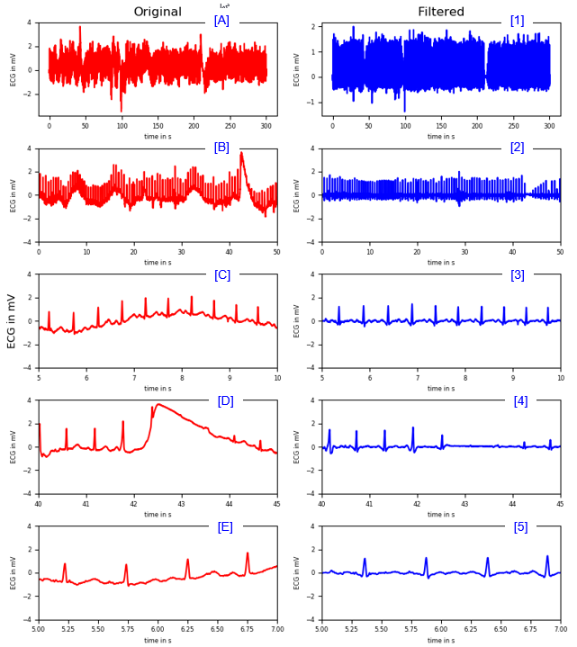
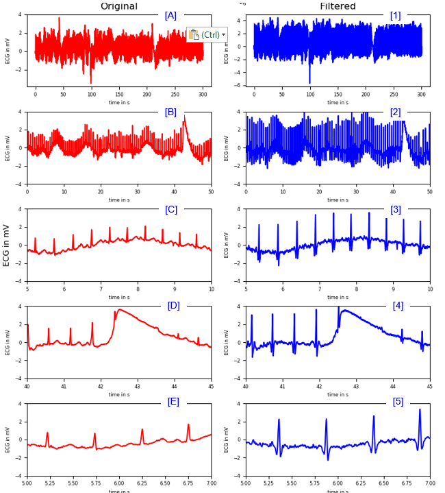
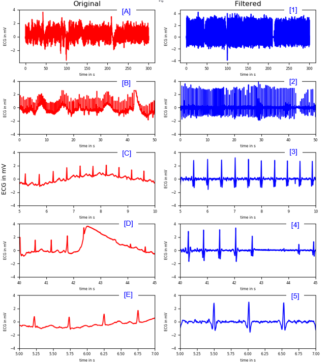
#                                                        PROCESSING                                                    #   

################################################################

n = 101;

a = 1;

ftap = signal.firwin(n,cutoff = [0.007,0.05], window = "hamming");

xf = signal.lfilter(ftap, a, x);

ftap = signal.firwin(n,cutoff = 0.03, window = "hamming",pass_zero = False);

xf = signal.lfilter(ftap, a, xf);

################################################################

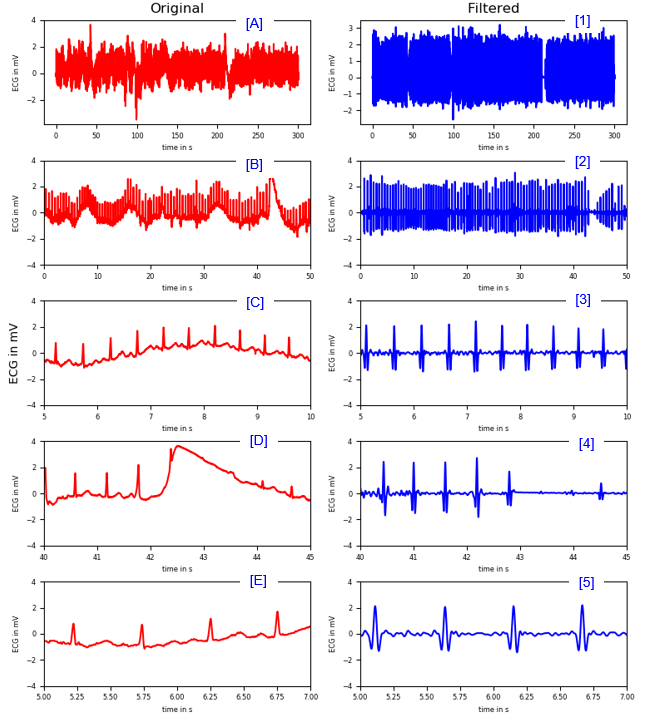
#                                                        PROCESSING                                                    #   

################################################################

n = 101;

a = 1;

ftap = signal.firwin(n,cutoff = [0.007,0.05], window = "hamming");

xf = signal.lfilter(ftap, a, x);

ftap = signal.firwin(n,cutoff = 0.03, window = "hamming",pass_zero = False);

xf = signal.lfilter(ftap, a, xf);

ftap = signal.firwin(n,cutoff = 0.15, window = "hamming");

xf = signal.lfilter(ftap, a, xf);

import numpy as np

import matplotlib.pyplot as plt

import scipy as sp

import scipy.misc as spm

from scipy.fftpack import fft

from scipy import signal

from scipy.signal import find_peaks

fs = 360;

fn = fs / 2; # Nyquist Frequency

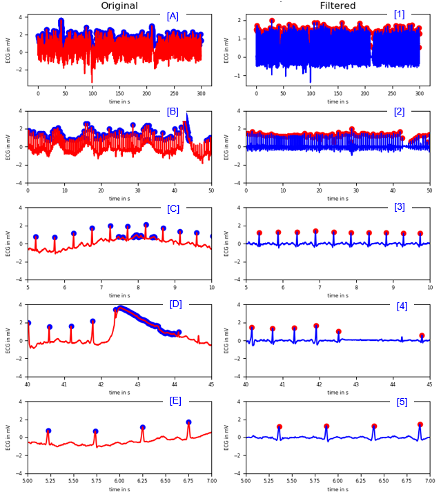
x = spm.electrocardiogram();

t = np.linspace(0,x.size-1,x.size) / fs;

f = np.linspace(0,x.size-1,x.size) * (fs / x.size);

peaks_x,_ = find_peaks(x, height = 0.7);

n = 101;

a = 1;

ftap = signal.firwin(n,cutoff = 0.03, window = "hamming",pass_zero = False);

xf = signal.lfilter(ftap, a, x);

peaks_xf,_ = find_peaks(xf, height = 0.5);

#######################################################

#                                              PLOT                                                     #   

#######################################################

FontSize_Xlabel = 6;

FontSize_Ylabel = 6;

bw = 0.40;

bh = 0.145;

bx = 0.025;

by = 0.1;

bx_gap = 0.075;

by_gap = 0.05;

by_shift = -0.05;

bx_shift = 0.05;

pltRegion1 = [bx + 0 * (bw + bx_gap) + bx_shift,by + 4*(by_gap + bh) + by_shift, bw, bh];

pltRegion2 = [bx + 0 * (bw + bx_gap) + bx_shift,by + 3*(by_gap + bh) + by_shift, bw, bh];

pltRegion3 = [bx + 0 * (bw + bx_gap) + bx_shift,by + 2*(by_gap + bh) + by_shift, bw, bh];

pltRegion4 = [bx + 0 * (bw + bx_gap) + bx_shift,by + 1*(by_gap + bh) + by_shift, bw, bh];

pltRegion5 = [bx + 0 * (bw + bx_gap) + bx_shift,by + 0*(by_gap + bh) + by_shift, bw, bh];

pltRegion6 = [bx + 1 * (bw + bx_gap) + bx_shift,by + 4*(by_gap + bh) + by_shift, bw, bh];

pltRegion7 = [bx + 1 * (bw + bx_gap) + bx_shift,by + 3*(by_gap + bh) + by_shift, bw, bh];

pltRegion8 = [bx + 1 * (bw + bx_gap) + bx_shift,by + 2*(by_gap + bh) + by_shift, bw, bh];

pltRegion9 = [bx + 1 * (bw + bx_gap) + bx_shift,by + 1*(by_gap + bh) + by_shift, bw, bh];

pltRegion10 = [bx + 1 * (bw + bx_gap) + bx_shift,by + 0*(by_gap + bh) + by_shift, bw, bh];

fig = plt.figure();

ax1 = fig.add_axes(pltRegion1);

ax2 = fig.add_axes(pltRegion2);

ax3 = fig.add_axes(pltRegion3);

ax4 = fig.add_axes(pltRegion4);

ax5 = fig.add_axes(pltRegion5);

ax6 = fig.add_axes(pltRegion6);

ax7 = fig.add_axes(pltRegion7);

ax8 = fig.add_axes(pltRegion8);

ax9 = fig.add_axes(pltRegion9);

ax10 = fig.add_axes(pltRegion10);

ax = ax1;

ax.plot(t, x,'r-');

ax.scatter(t[peaks_x],x[peaks_x],c='blue');

ax.set_xlabel('time in s', fontsize = FontSize_Xlabel );

ax.set_ylabel('ECG in mV', fontsize = FontSize_Ylabel );

ax.tick_params(axis='both' ,which='major', labelsize = 6);

ax.set_title("Original");

ax = ax2;

ax.plot(t, x,'r-');

ax.scatter(t[peaks_x],x[peaks_x],c='blue');

ax.set_xlim(0.0,50);

ax.set_ylim(-4,4);

ax.set_xlabel('time in s', fontsize = FontSize_Xlabel );

ax.set_ylabel('ECG in mV', fontsize = FontSize_Ylabel );

ax.tick_params(axis='both' ,which='major', labelsize = 6);

ax = ax3;

ax.plot(t, x,'r-');

ax.scatter(t[peaks_x],x[peaks_x],c='blue');

ax.set_xlim(5.0,10.0);

ax.set_ylim(-4,4);

ax.set_xlabel('time in s', fontsize = FontSize_Xlabel );

ax.set_ylabel('ECG in mV', fontsize = FontSize_Ylabel );

ax.tick_params(axis='both' ,which='major', labelsize = 6);

ax = ax4;

ax.plot(t, x,'r-');

ax.scatter(t[peaks_x],x[peaks_x],c='blue');

ax.set_xlim(40.0,45.0);

ax.set_ylim(-4,4);

ax.set_xlabel('time in s', fontsize = FontSize_Xlabel );

ax.set_ylabel('ECG in mV', fontsize = FontSize_Ylabel );

ax.tick_params(axis='both' ,which='major', labelsize = 6);

ax = ax5;

ax.plot(t, x,'r-');

ax.scatter(t[peaks_x],x[peaks_x],c='blue');

ax.set_xlim(5.0,7.0);

ax.set_ylim(-4,4);

ax.set_xlabel('time in s', fontsize = FontSize_Xlabel );

ax.set_ylabel('ECG in mV', fontsize = FontSize_Ylabel );

ax.tick_params(axis='both' ,which='major', labelsize = 6);

ax = ax6;

ax.plot(t,xf,'b-');

ax.scatter(t[peaks_xf],xf[peaks_xf],c='red');

ax.set_xlabel('time in s', fontsize = FontSize_Xlabel );

ax.set_ylabel('ECG in mV', fontsize = FontSize_Ylabel );

ax.tick_params(axis='both' ,which='major', labelsize = 6);

ax.set_title("Filtered");

ax = ax7;

ax.plot(t, xf,'b-');

ax.scatter(t[peaks_xf],xf[peaks_xf],c='red');

ax.set_xlim(0.0,50);

ax.set_ylim(-4,4);

ax.set_xlabel('time in s', fontsize = FontSize_Xlabel );

ax.set_ylabel('ECG in mV', fontsize = FontSize_Ylabel );

ax.tick_params(axis='both' ,which='major', labelsize = 6);

ax = ax8;

ax.plot(t, xf,'b-');

ax.scatter(t[peaks_xf],xf[peaks_xf],c='red');

ax.set_xlim(5.0,10.0);

ax.set_ylim(-4,4);

ax.set_xlabel('time in s', fontsize = FontSize_Xlabel );

ax.set_ylabel('ECG in mV', fontsize = FontSize_Ylabel );

ax.tick_params(axis='both' ,which='major', labelsize = 6);

ax = ax9;

ax.plot(t, xf,'b-');

ax.scatter(t[peaks_xf],xf[peaks_xf],c='red');

ax.set_xlim(40.0,45.0);

ax.set_ylim(-4,4);

ax.set_xlabel('time in s', fontsize = FontSize_Xlabel );

ax.set_ylabel('ECG in mV', fontsize = FontSize_Ylabel );

ax.tick_params(axis='both' ,which='major', labelsize = 6);

ax = ax10;

ax.plot(t, xf,'b-');

ax.scatter(t[peaks_xf],xf[peaks_xf],c='red');

ax.set_xlim(5.0,7.0);

ax.set_ylim(-4,4);

ax.set_xlabel('time in s', fontsize = FontSize_Xlabel );

ax.set_ylabel('ECG in mV', fontsize = FontSize_Ylabel );

ax.tick_params(axis='both' ,which='major', labelsize = 6);

plt.gcf().set_size_inches(8.0,9);

fig.show();

import numpy as np

import matplotlib.pyplot as plt

import scipy as sp

import scipy.misc as spm

from scipy.fftpack import fft

from scipy import signal

from scipy.signal import find_peaks

fs = 360;

fn = fs / 2; # Nyquist Frequency

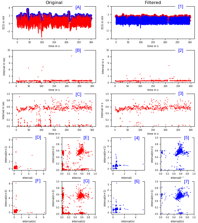
x = spm.electrocardiogram();

t = np.linspace(0,x.size-1,x.size) / fs;

f = np.linspace(0,x.size-1,x.size) * (fs / x.size);

peaks_x,_ = find_peaks(x, height = 0.7);

t_peak_x = t[peaks_x];

w = [1,-1];

x_peak_interval = np.convolve(t_peak_x,w,mode='same');

n = 101;

a = 1;

ftap = signal.firwin(n,cutoff = 0.03, window = "hamming",pass_zero = False);

xf = signal.lfilter(ftap, a, x);

peaks_xf,_ = find_peaks(xf, height = 0.5);

t_peak_xf = t[peaks_xf];

w = [1,-1];

xf_peak_interval = np.convolve(t_peak_xf,w,mode='same');

#######################################################

#                                              PLOT                                                     #   

#######################################################

FontSize_Xlabel = 7;

FontSize_Ylabel = 7;

bw = 0.40;

bh = 0.145;

bx = 0.025;

by = 0.1;

bx_gap = 0.075;

by_gap = 0.05;

by_shift = -0.05;

bx_shift = 0.05;

pltRegion1 = [bx + 0 * (bw + bx_gap) + bx_shift,by + 4*(by_gap + bh) + by_shift, bw, bh];

pltRegion2 = [bx + 0 * (bw + bx_gap) + bx_shift,by + 3*(by_gap + bh) + by_shift, bw, bh];

pltRegion3 = [bx + 0 * (bw + bx_gap) + bx_shift,by + 2*(by_gap + bh) + by_shift, bw, bh];

pltRegion4 = [bx + 0 * (bw + bx_gap) + bx_shift,by + 1*(by_gap + bh) + by_shift, 0.4*bw, bh];

pltRegion5 = [bx + 0.5 * (bw + bx_gap) + bx_shift,by + 1*(by_gap + bh) + by_shift, 0.4*bw, bh];

pltRegion6 = [bx + 0 * (bw + bx_gap) + bx_shift,by + 0*(by_gap + bh) + by_shift, 0.4*bw, bh];

pltRegion7 = [bx + 0.5 * (bw + bx_gap) + bx_shift,by + 0*(by_gap + bh) + by_shift, 0.4*bw, bh];

pltRegion8 = [bx + 1 * (bw + bx_gap) + bx_shift,by + 4*(by_gap + bh) + by_shift, bw, bh];

pltRegion9 = [bx + 1 * (bw + bx_gap) + bx_shift,by + 3*(by_gap + bh) + by_shift, bw, bh];

pltRegion10 = [bx + 1 * (bw + bx_gap) + bx_shift,by + 2*(by_gap + bh) + by_shift, bw, bh];

pltRegion11 = [bx + 1 * (bw + bx_gap) + bx_shift,by + 1*(by_gap + bh) + by_shift, 0.4*bw, bh];

pltRegion12 = [bx + 1.5 * (bw + bx_gap) + bx_shift,by + 1*(by_gap + bh) + by_shift, 0.4*bw, bh];

pltRegion13 = [bx + 1 * (bw + bx_gap) + bx_shift,by + 0*(by_gap + bh) + by_shift, 0.4*bw, bh];

pltRegion14 = [bx + 1.5 * (bw + bx_gap) + bx_shift,by + 0*(by_gap + bh) + by_shift, 0.4*bw, bh];

fig = plt.figure();

ax1 = fig.add_axes(pltRegion1);

ax2 = fig.add_axes(pltRegion2);

ax3 = fig.add_axes(pltRegion3);

ax4 = fig.add_axes(pltRegion4);

ax5 = fig.add_axes(pltRegion5);

ax6 = fig.add_axes(pltRegion6);

ax7 = fig.add_axes(pltRegion7);

ax8 = fig.add_axes(pltRegion8);

ax9 = fig.add_axes(pltRegion9);

ax10 = fig.add_axes(pltRegion10);

ax11 = fig.add_axes(pltRegion11);

ax12 = fig.add_axes(pltRegion12);

ax13 = fig.add_axes(pltRegion13);

ax14 = fig.add_axes(pltRegion14);

cList = ['red','blue','green','black','m'];

lList = ['r-','b-','g-','k-','m-'];

ax = ax1;

ax.plot(t, x,'r-');

ax.scatter(t[peaks_x],x[peaks_x],c='blue');

ax.set_xlabel('time in s', fontsize = FontSize_Xlabel );

ax.set_ylabel('ECG in mV', fontsize = FontSize_Ylabel );

ax.tick_params(axis='both' ,which='major', labelsize = 6);

ax.set_title("Original");

ax = ax2;

ax.scatter(t_peak_x, x_peak_interval,s=1,c='red');

ax.set_ylim([0,10]);

ax.set_xlabel('time in s', fontsize = FontSize_Xlabel );

ax.set_ylabel('Interval in sec', fontsize = FontSize_Ylabel );

ax.tick_params(axis='both' ,which='major', labelsize = 6);

ax = ax3;

ax.scatter(t_peak_x, x_peak_interval,s=1,c='red');

ax.set_ylim([0,1]);

ax.set_xlabel('time in s', fontsize = FontSize_Xlabel );

ax.set_ylabel('Interval in sec', fontsize = FontSize_Ylabel );

ax.tick_params(axis='both' ,which='major', labelsize = 6);

ax = ax4;

ax.scatter(x_peak_interval[1:], np.roll(x_peak_interval,1)[1:],s=1,c='red');

ax.set_xlabel('interval(n)', fontsize = FontSize_Xlabel );

ax.set_ylabel('interval(n+1)', fontsize = FontSize_Ylabel );

ax.tick_params(axis='both' ,which='major', labelsize = 6);

ax = ax5;

ax.scatter(x_peak_interval[1:], np.roll(x_peak_interval,1)[1:],s=1,c='red');

ax.set_xlim([0,1]);

ax.set_ylim([0,1]);

ax.set_xlabel('interval(n)', fontsize = FontSize_Xlabel );

ax.set_ylabel('interval(n+1)', fontsize = FontSize_Ylabel );

ax.tick_params(axis='both' ,which='major', labelsize = 6);

ax = ax6;

ax.scatter(x_peak_interval[2:], np.roll(x_peak_interval,2)[2:],s=1,c='red');

ax.set_xlabel('interval(n)', fontsize = FontSize_Xlabel );

ax.set_ylabel('interval(n+2)', fontsize = FontSize_Ylabel );

ax.tick_params(axis='both' ,which='major', labelsize = 6);

ax = ax7;

ax.scatter(x_peak_interval[2:], np.roll(x_peak_interval,2)[2:],s=1,c='red');

ax.set_xlim([0,1]);

ax.set_ylim([0,1]);

ax.set_xlabel('interval(n)', fontsize = FontSize_Xlabel );

ax.set_ylabel('interval(n+2)', fontsize = FontSize_Ylabel );

ax.tick_params(axis='both' ,which='major', labelsize = 6);

ax = ax8;

ax.plot(t, xf,'b-');

ax.scatter(t[peaks_xf],xf[peaks_xf],c='red');

ax.set_ylim(-4,4);

ax.set_xlabel('time in s', fontsize = FontSize_Xlabel );

ax.set_ylabel('ECG in mV', fontsize = FontSize_Ylabel );

ax.tick_params(axis='both' ,which='major', labelsize = 6);

ax.set_title("Filtered");

ax = ax9;

ax.scatter(t_peak_xf, xf_peak_interval,s=1,c='red');

ax.set_ylim([0,10]);

ax.set_xlabel('time in s', fontsize = FontSize_Xlabel );

ax.set_ylabel('Interval in s', fontsize = FontSize_Ylabel );

ax.tick_params(axis='both' ,which='major', labelsize = 6);

ax = ax10;

ax.scatter(t_peak_xf, xf_peak_interval,s=1,c='red');

ax.set_ylim([0,1]);

ax.set_xlabel('time in s', fontsize = FontSize_Xlabel );

ax.set_ylabel('Interval in s', fontsize = FontSize_Ylabel );

ax.tick_params(axis='both' ,which='major', labelsize = 6);

ax = ax11;

ax.scatter(xf_peak_interval[1:], np.roll(xf_peak_interval,1)[1:],s=1,c='blue');

ax.set_xlabel('interval(n)', fontsize = FontSize_Xlabel );

ax.set_ylabel('interval(n+1)', fontsize = FontSize_Ylabel );

ax.tick_params(axis='both' ,which='major', labelsize = 6);

ax = ax12;

ax.scatter(xf_peak_interval[1:], np.roll(xf_peak_interval,1)[1:],s=1,c='blue');

ax.set_xlim([0,1]);

ax.set_ylim([0,1]);

ax.set_xlabel('interval(n)', fontsize = FontSize_Xlabel );

ax.set_ylabel('interval(n+1)', fontsize = FontSize_Ylabel );

ax.tick_params(axis='both' ,which='major', labelsize = 6);

ax = ax13;

ax.scatter(xf_peak_interval[2:], np.roll(xf_peak_interval,2)[2:],s=1,c='blue');

ax.set_xlabel('interval(n)', fontsize = FontSize_Xlabel );

ax.set_ylabel('interval(n+1)', fontsize = FontSize_Ylabel );

ax.tick_params(axis='both' ,which='major', labelsize = 6);

ax = ax14;

ax.scatter(xf_peak_interval[2:], np.roll(xf_peak_interval,2)[2:],s=1,c='blue');

ax.set_xlim([0,1]);

ax.set_ylim([0,1]);

ax.set_xlabel('interval(n)', fontsize = FontSize_Xlabel );

ax.set_ylabel('interval(n+1)', fontsize = FontSize_Ylabel );

ax.tick_params(axis='both' ,which='major', labelsize = 6);

plt.gcf().set_size_inches(8.0,9);

fig.show();