This page is to show how to implement single perceptron using Matlab Deep Learning Toolbox. This is not about explaining on theory / mathematical procedure of Perceptron. For mathematical background of single perceptron, I wrote a separate page for it. If you are completely new to neural network, I would suggest you to go through single perceptron page first. If you are already familiar with neural network concept, but new to Matlab Deep Learning package, I would suggest you to take a loot at this note first.
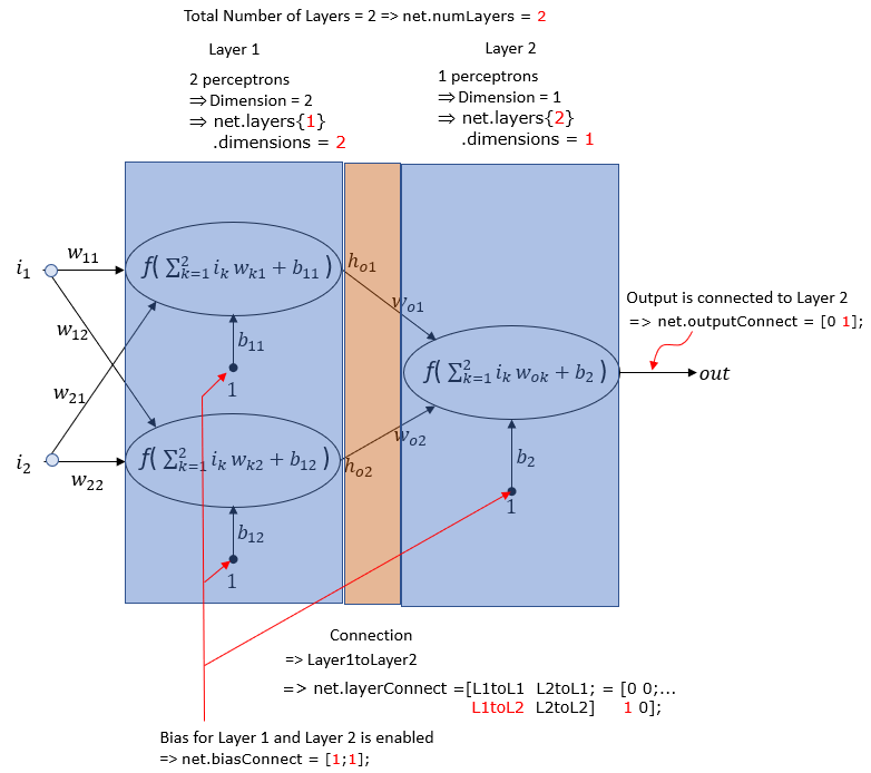
In this note, we will talk about how to implement following network (2 layer perceptron as shown below) with Matlab Deep Learning toolbox.
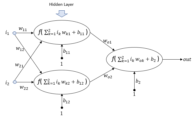
Comparing to single perceptron case, the complexity of the code and required setting gets much complicated and I spent a lot of time for try and error. With help of Mathworks engineer, finally I figured out how to configure a simple MLP(Multi Layer Perceptron) network and I summarized the key parameters setting as an illustration as shown below.
Followings shows parameter setting to create a MLP with one hidden layer and configure/initialize each components.
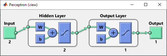
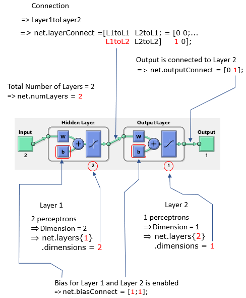
If you run the script, Matlab draws the network structure as shown below and I labeled each component with Matlab Deep learning parameter. Compare this one with the one shown above. Usually when you first design a network, you may design a network as shown above since it is more of standard way of description and then translate it into Matlab style network structure. You should be familiar with switching back and forth between the two different way of representation.
Examples
Example 01 >
|
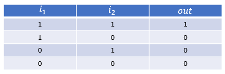
pList = [1 1 0 0; 1 0 1 0]; tList = [0 1 1 0];
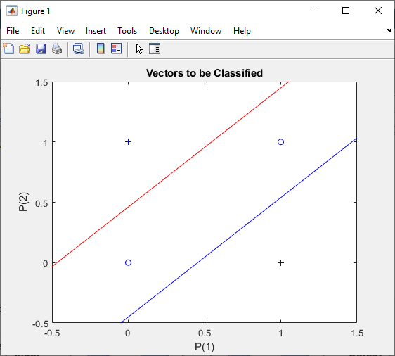
plotpv(pList,tList);
net = perceptron; net.performFcn = 'mse'; net.trainFcn = 'trainlm';
net.numLayers = 2;
net.layers{1}.name = 'Hidden Layer'; %net.layers{1}.transferFcn = 'hardlim'; net.layers{1}.transferFcn = 'tansig'; net.layers{1}.dimensions = 2;
net.layers{2}.name = 'Output Layer'; %net.layers{2}.transferFcn = 'hardlim'; net.layers{2}.transferFcn = 'tansig'; net.layers{2}.dimensions = 1;
net.layerConnect = [0 0;... 1 0]; net.outputConnect = [0 1]; net.biasConnect = [1;1];
net = configure(net,[0; 0],[0]);
net.b{1} = [1 1]'; net.b{2} = 1; wi = [1 -0.8; 1 -0.8]; net.IW{1,1} = wi; wo = [1 -0.8]; net.LW{2,1} = wo;
view(net);
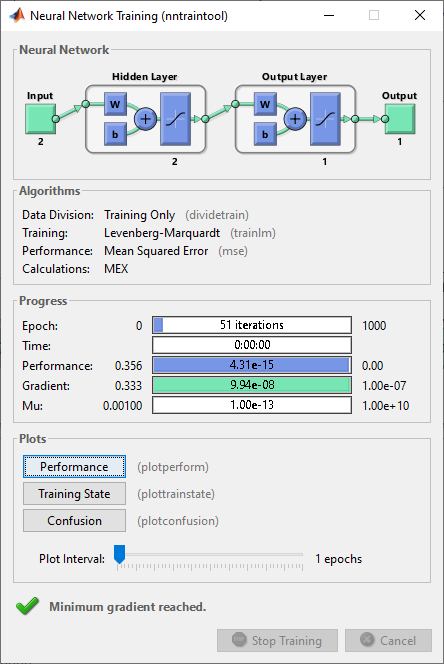
[net,tr] = train(net,pList,tList);
plotpc(net.IW{1,1},net.b{1}) axis([-0.5 1.5 -0.5 1.5]);
y = net(pList) |
|
|
|
|